If you have trouble viewing this, try the pdf of this post. You can download the code used to produce the figures in this post.
Image SNR with energy-selective detectors
This is the last post in my series discussing my paper, “Near optimal energy selective x-ray imaging system performance with simple detectors”[2]. In the last post I showed plots of the signal to noise ratio (SNR) of images with different types of energy-selective detectors. In this post, I show images illustrating these differences. These images were not included in the paper but they are based on its approach. The images are calculated from a random sample of the energy spectrum at each point in a projection image. These data are then used to make images with (a) the total energy, which are comparable to the detectors now used in commercial systems, (b) the total number of photons, (c) an N2Q detector, and (d) an optimal full spectrum by weighting the spectrum data before summing, as described in Tapiovaara and Wagner (TW)[3]. I use the theory developed in my paper, to make images from A-space data using data from the N2Q detector. In order to do this, I need an estimator that achieves the Cramèr-Rao lower bound (CRLB). For this I use the A-table estimator I introduced in my paper “Estimator for photon counting energy selective x-ray imaging with multibin pulse height analysis”[1] available for download here.
The Monte Carlo experiment
The experimental set up is shown in Fig. 1↓ and the details are described in the caption. Poisson distributed random data are computed with expected value equal to the transmitted spectrum at each pixel. The random data are stored in a matrix with number of rows equal to the number of pixels in the image and number of columns equal to the number of energies in the spectrum. The matrix is used to compute the data for the images. For example, the photon count image is the sum of each of the rows. This gives a column vector, that can be “re-shaped” to form the image. Similarly, the N2Q data can be generated by summing along the rows from the lowest energy to the threshold energy, which is the red, dashed, vertical line shown in the exit spectrum in the bottom panel, and from the threshold energy plus one to the highest energy. This gives the N2 data at each row. The Q data is the sum of the photon counts each multiplied by the energy for that point in the spectrum.
The simulated object was generated with my sim2d.m function, which is included with the code package. The relevant code from P36SNRimages.m is in Listing 2↓
%% init the simulated object
1thicknesses = [1 -.1 .1]; % gm/cm^2 — will assume density is equal to 1 2nx = 256; ny = 256; 3zsiz = nx + 1i*ny; % dimensions of images 4z1 = 1 + 1i; 5 % boxes coords in unit based coords 6zcorners = nx*[ 7 .1*z1, .9*z1; % background material region 8 .2*z1,.2*z1 + .2+.6i; 9 .2*z1,.2*z1 + .2+.6i; % hole for feature 10 ]; 11 % make object out of 3 planes: background, 12 % -feature from background slab, 13 % fill in feature material in background slab 14tplanes = zeros(ny,nx,2); % one plane per background and feature 15 % combine background plane with hole for feature 16for kt = 1:2 17 timg = sim2d(zsiz,’rect’,[zcorners(kt,:),thicknesses(kt)]); 18 tplanes(:,:,1) = tplanes(:,:,1) + timg; 19end 20% add in feature 21tplanes(:,:,2) = sim2d(zsiz,’rect’,[zcorners(3,:),thicknesses(3)]); 22 % reformat into columns (ny*nx,2) 23ts_object = reshape(tplanes,ny*nx,2); 24
The object, shown in the middle part of Fig. 1↓ on the right, is generated as three planes that are summed pixel by pixel to form it. The three planes are the overall background material slab, a hole in the background for the feature and the feature alone. The code from lines 1-11 of Listing 2↑ defines the sim2D.m specifications for the image in each plane. See the “help” for sim2D.m for more details on the specification. The tplanes 3D array holds the background and feature thicknesses in each plane respectively. This is computed in lines 12-22. The last line, 24, reshapes tplanes so each row is the thickness of the feature and background material.
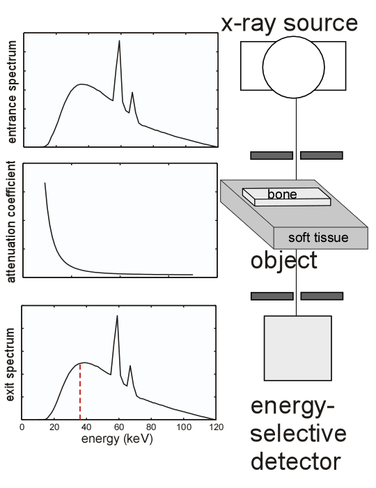
Figure 1 Block diagram of the experiment. An x-ray tube generates the entrance spectrum. The collimated beam goes through every pixel of the object with “good geometry” so scatter is negligible. The object consists of the background, a slab of tissue material, and the feature, a box of bone-material. The feature is embedded in the background so there is a hole in the tissue slab to fit the bone box. The background is 1 gm ⁄ cm2 and the feature is 0.1 gm ⁄ cm2. The transmitted spectrum is measured at each point in the image.
The random transmitted spectrum is generated using the code shown in Listing 2↓ below.
%% make the incident spectrum and transmitted spectrum
1kV = 120; 2[dum,dum,specdat] = XrayTubeSpectrumTasmip(kV,’number_spectrum’,’clipzeros’); 3specdat.mus = [xraymu(ztback,specdat.egys) xraymu(ztfeat,specdat.egys)]; 4 5%% make the random transmitted data 6transmission = exp(-ts_object*specdat.mus’); 7 % the expected values of the transmitted spectrum 8lambdas = bsxfun(@times,transmission,specdat.specnum_norm’); % siz = (ny*nx,nenergy) 9N = 10^3; % total number of photons in trasnmitted spectrum 10offset2counts = 1/numel(specdat.egys); % add small number so no zeros 11 % generate the random data 12ns = poissrnd(N*lambdas) + offset2counts; 13
The spectrum and the attenuation coefficients of the background and feature material are computed in lines 1-4. The expected values of the transmitted spectrum are generated in lines 6-10. The random data are computed in line 13. The ns matrix has one row per pixel in the image and the columns are the values for each spectrum energy. Note that a small constant is added to the data so there are no zero values. This would lead to problems in the computation of the log data for the N2Q image.
Making the N, Q, and optimal, full-spectrum images
The N, Q, and optimal, full-spectrum TW images were computed directly from the random transmitted data generated with the code in Listing 2↑. The code to generate the images is in Listing 3↓. The bsxfun function is a fast way to compute element-by-element products of a matrix and a vector (see the Matlab help).
%% N image
1Ns = sum(ns,2); 2imdatN = reshape(Ns,ny,nx); 3snrN = SNRfeature(imdatN); 4 5%% Q image 6Qs = sum(bsxfun(@times,ns,specdat.egys’),2); 7imdatQ = reshape(Qs,ny,nx); 8snrQ = SNRfeature(imdatQ); 9 10%% Make the TW optimal image by weighting the full spectrum data at each point in image 11 % for a thin object, the optimal weighting function is proportional to 12 % diff of the mus at each energy 13dmus = diff(specdat.mus,1,2); 14dmus_norm = dmus/sum(dmus); 15imTW = reshape(sum(bsxfun(@times,ns,dmus_norm’),2),ny,nx); 16snrTW = SNRfeature(imTW); 17
Making the N2Q data
Computing the N2Q image is more complex but the result has advantages over the other images including the full-spectrum TW. It is a two step process: first, compute the A-vector data, then compute a low-noise image from the A-vectors. I will discuss the first step in this section and leave the computation of the image for the next section. The steps to compute the A-vector data are (each step refers to the lines of code in Listing 4↓):
- Compute the N2Q data from the ns matrix and the threshold index (1-5)
- Make the “air data” i.e. the expected value of the data with no object in the beam (6-9).
- Compute − log(N2Q⁄N2Q0) (10-12)
- Compute noise-free calibration data for a two element step wedge made of the background and feature material. Use of these materials is unrealistic but the results would be the same for more realistic materials such as aluminum and plastic and would make the code needlessly complex. (14-28)
- Compute the covariance of the log data. This is required for the A-table algorithm. This can be done experimentally from the log N2Q image using the same approach. (30-31)
- Solve for the A-vector image using my AtableSolveEquations.m function. This is included with the code package. (33-38)
1%% N2Q data — will process using my A-table method 2 % first compute object data 3Ethreshold = 35; % keV 4[dum,idxthreshold] = min(abs(specdat.egys - Ethreshold)); 5N2Qs = [sum(ns(:,1:idxthreshold),2) sum(ns(:,(idxthreshold+1):end),2) Qs]; 6 % ’air data’ i.e. no object in beam. Assume has no noise 7N2Qs0 = N*[sum(specdat.specnum_norm(1:idxthreshold)) ... 8 sum(specdat.specnum_norm((idxthreshold+1):end)) ... 9 sum(specdat.specnum_norm.*specdat.egys)]; 10 % add offset to air data so it matches the offset added to noisy data 11N2Qs0(1:2) = N2Qs0(1:2) + offset2counts; 12logN2Qs = bsxfun(@minus,log(N2Qs0),log(N2Qs)); % these are positive numbers 13 14%% calibration data — assume noise free 15ncalib_points = 20; 16t1s_calib = linspace(-.5,4*thicknesses(1),ncalib_points); % allow negatives so fewer out of range points 17t2s_calib = linspace(-.3,4*thicknesses(3),ncalib_points); 18idxs = combinator(ncalib_points,2,’p’,’r’); % permutations taken 2 at a time with repitition 19ts_calib = [t1s_calib(idxs(:,1))’ t2s_calib(idxs(:,2))’]; 20transmission_calib = exp(-ts_calib*specdat.mus’); 21lambdas_calib = bsxfun(@times,transmission_calib,specdat.specnum_norm’); % siz = (ncalib steps,nenergy) 22ns_calib = N*lambdas_calib + offset2counts; % no noise for calibration data 23Qs_calib = sum(bsxfun(@times,ns_calib,specdat.egys’),2); 24N2Qs_calib = [sum(ns_calib(:,1:idxthreshold),2) sum(ns_calib(:,(idxthreshold+1):end),2) Qs_calib]; 25 % air data does not change so use results from previous cell 26logN2Qs_calib = bsxfun(@minus,log(N2Qs0),log(N2Qs_calib)); % these are positive numbers 27cdat.As = ts_calib; 28cdat.logI = logN2Qs_calib; 29 30%% compute covariance of log(N2Q) data from background region of image 31covstats.RL = cov(logN2Qs(idxs4back,:)); 32 33%% solve for A vector image data 34tdat.As = ts_object; 35tdat.logI = logN2Qs; 36% N2Qdat = PolyASolveEquations(cdat,tdat); 37N2Qdat = AtableSolveEquations(cdat,tdat,’stats’,covstats); 38zAs_back = zcomp(N2Qdat.Astest(idxs4back,:)); 39
The final steps are to compute a low noise image from the A-vector data. This is discussed in the next section.
Compute low-noise image from N2Q A-vector data
The output of the A-space method is a set of A-vectors for every pixel in the image or line in CT. We can make a scalar image comparable to the other images by doing a vector dot product of the A-vector at every pixel with a unit vector. This is called a generalized projection. By varying the angle of the unit vector, we can cancel tissues from images or make images comparable to a conventional projection image. This was first discussed in Section 4.6 of my dissertation and in more detail in Sections 2.2 and 2.3 of this paper available on my website.
A problem with forming images from A-vector data is that the noise is highly negatively correlated. As a result, the noise will depend on the angle of the unit vector. My my paper described an alternate approach, which solved this problem. The approach is to transform with data by using a whitening transform. My paper showed that with this approach, you can make images with the best SNR available for a given detector type.
Whitening transforms in general are described in one of my previous posts, which is available in Ch. 25 of my ebook. The whitening transform is computed with the code in Listing 5↓. Line 2 computes the A-vector covariance from the data in the background region. Line 3 computes the transform and line 4 applies it to the whole image. Line 5 converts the whitened image data to complex numbers to make it easy for the following computations
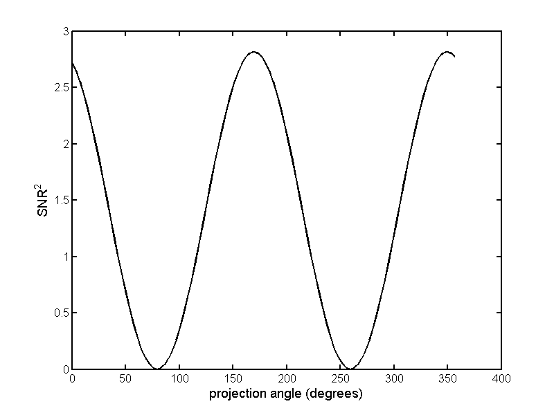
Once we have the whitened data, we can compute images by taking a vector dot product with a unit vector at each pixel and choose the angle of the unit vector to maximize the SNR. This is done with the code in Listing 5↓. The angle for maximum SNR is chosen by computing multiple images for a large number of angles from 0 to 2π and selecting the one that gives the maximum value. Fig. 2↓ plots the results.
1%% find projection angle for maximum SNR 2nprojangles = 100; 3projangles = linspace(0,2*pi,nprojangles+1); % will remove 1 so no wraparound 4projangles = projangles(1:nprojangles); 5snrs = zeros(nprojangles,1); 6 7for kangle = 1:nprojangles 8 improj = zdot(zAswhiten,exp(1i*projangles(kangle))); 9 snrs(kangle) = SNRfeature(improj); 10end 11idxpeak = findpeaks(snrs); 12assert(~isempty(idxpeak)); 13imN2Q = reshape(zdot(zAswhiten,exp(1i*projangles(idxpeak(1)))),ny,nx); 14snrN2Q = SNRfeature(imN2Q);
Results
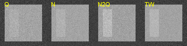
The images with different detectors are shown in Fig. 3↓. These were all computed from the same random data; the only difference is the processing to emulate the characteristics of each detector type. As expected from the results in the last post, the Q image has the lowest SNR, the N is somewhat better and the N2Q is close to the Tapiovaara-Wagner SNR. The N2Q and TW images have different visual appearance with the N2Q seeming to have higher contrast but the numerical value of the N2Q image SNR is close to the TW image.

Conclusions
The N2Q detector with A-space processing has SNR close to the TW optimal. I showed in my paper that images with high SNR can also be computed from N2 (two-bin PHA) and NQ (simultaneous photon counts and integrated energy) detectors. The fact that these low energy-resolution detectors give such good performance is due to the simplicity of the underlying information, which can be completely summarized by the coefficients of two basis functions. This information was not used by Tapiovaara and Wagner or other people who have used their approach.
Notice that there are generalized projection angles in Fig. 2↑ with 0 SNR. These are the angles that cancel the feature material from the image. The images, computed from the whitened data, with zero SNR angles for the feature and background materials respectively, are shown in Fig. 4↑. With the A-space method, we not only get high SNR images but also have the additional A-space information that we can use for selective material imaging. This is not possible with the Tapiovaara-Wagner approach.
--Bob Alvarez
Last edited Apr 13, 2013
Copyright © 2013 by Robert E. Alvarez
Linking is allowed but reposting or mirroring is expressly forbidden.
References
[1] : “Estimator for Photon Counting Energy Selective X-ray Imaging with Multi-bin Pulse Height Analysis”, Med. Phys., pp. 2324—2334, 2011.
[2] : “Near optimal energy selective x-ray imaging system performance with simple detectors”, Med. Phys., pp. 822—841, 2010.
[3] : “SNR and DQE analysis of broad spectrum X-ray imaging”, Phys. Med. Biol., pp. 519—529, 1985.