If you have trouble viewing this, click here for a pdf of this post. See also this article for a more complete discussion of the dimensionality of attenuation coefficients.
The dimensionality of attenuation coefficients
In my previous post, I showed how the singular value decomposition (SVD) can be used to study the effective rank of a matrix. In this post, I use the SVD to quantify the dimensionality of attenuation coefficients.
The idea is simple:
- compute the attenuation coefficients of the elements found in body materials at a fixed set of energies.
- place the attenuation coefficient samples as the columns of a matrix
- compute the SVD of the matrix
- the principal values are the squares of the singular values divided by the number of energies
- the dimensionality of the space is the number of significant principal values.
In order to do this, we need to answer several questions:
- What elements to use? ICRU report 44[1] gives the elements and fractions by weight of common body materials so I used the set of elements found in cortical bone and soft tissue. I also analyzed the case of an externally administered contrast agent which contains iodine. The K-edge of iodine is near 33 keV, which is within the diagnostic region, so it requires a larger number of basis functions to represent it.
- How to weight the individual elements? From linear algebra, multiplying a column (or row) of a matrix by a constant does not affect the rank but it will affect the principal values since their sum is equal to the sum of the variances of the columns. The compositions from ICRU 44 have a wide distribution with hydrogen, carbon, and oxygen being the most prevalent and the higher atomic number elements much less common. Another issue is that the variation of the attenuation coefficient with energy depends strongly on the atomic number. The variation is much larger for higher atomic number so if we use equal weighting they would dominate the variance. In my analysis, I standardized each of the columns so they had unit standard deviation by subtracting the mean and dividing by the standard deviation. All the elements were treated equally so this somewhat over weights the high atomic numbers and overstates the dimensionality. Other choices will result in different principal values but I have not found that they affect the basic conclusions about the dimensionality.
- What set of energies to use? In general, we would expect that the larger the energy range the higher the effective dimensionality (see Fig. 2 of this post). The lower energy limit has the largest effect on the dimensionality since the cross-sections of the interactions have the largest variations at lower energy. The energy range used in diagnostic imaging is a practical compromise between information, which tends to be highest at lower energies, and dose, which tends to be lower at higher energy where the body attenuation is lower. In the analysis I used 100 energies equally spaced from 20 to 150 keV. Again, this tends to overstate the dimensionality since most diagnostic systems use a higher set of energies.
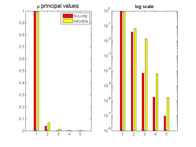
Fig. 1↓ shows the principal values for two cases. The first case (“bio-only”) I used the elements found in the normal body materials, bone and soft tissue. In the second case (“w/iodine”), I added the attenuation coefficient of iodine to the set of elements. The left panel shows a linear plot while the right panel uses a logarithmic scale. Notice that with the normal body materials, there is a sharp drop off of the values after the second. When iodine is included, the third principal value is significant but the fourth principal value is substantially smaller than the third.
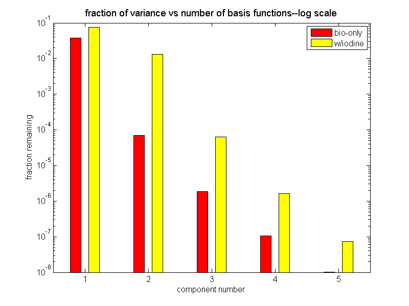
Another way to plot these values is to show the part of the variation remaining as a function of the number of basis functions. In the notation of this post, I plot
∥M − Ma∥2 = N⎲⎳i = r + 1d2i ⁄ N⎲⎳i = 1d2i
as a function of the rank r. Fig. 2↓ shows the results. Again it is clear that two functions represent most (0.9999) of the variation with ordinary body materials and three functions represent the same fraction (0.9999) when iodine is included.
Implications of low dimensionality
The low dimensionality of attenuation coefficients has important practical implications. First, it implies that we can summarize the complete attenuation coefficient function of energy with two numbers. That is, since f1(E) and f2(E) are known beforehand and
μ(E) = a1f1(E) + a2f2(E)
then the two numbers a1 and a2 carry all the information. These are the numbers that our imaging system needs to infer from the transmitted x-ray flux.
The low dimensionality also implies that we can use relatively simple methods to extract the energy information. In practice, measurements with two different spectra are sufficient. The results here show that these extract complete information. Using more spectra does not increase the information although in later posts I will show that these can be used to lower the noise in the processed data.
Another implication of the low dimensionality is that the information that we can extract is limited. For example, we cannot distinguish between more than two body materials. A third material will appear to be a combination of two other materials. But there are ways to process and display the energy information to extract very different information from that available from a conventional energy integrating system with no energy spectrum information.
Matlab code to compute the results in this post is available here.
Last edited July 16, 2011.
© 2011 by Aprend Technology and Robert E. Alvarez
Linking is allowed but reposting or mirroring is expressly forbidden.
References
[1] : Report 44: Tissue Substitutes in Radiation Dosimetry and Measurement. URL http://www.icru.org.