If you have trouble viewing this, try the pdf of this post. You can download the code used to produce the figures in this post.
The constant covariance approximation to the CRLB with pileup
In my last post, I showed that the probability distribution of photon counting detector data with pileup is multivariate normal for the counts typically used in material selective imaging. With the normal distribution and a linear model, the Cramèr-Rao lower bound (CRLB) for the covariance of the A-vector data includes a term that depends on the change in the measurement data covariance with A. Without pileup I show in this post and in the Appendix of my “Dimensionality and noise ...” paper[2], available for free download here, that the change in covariance term is negligible for large enough counts. In Appendix B of my “SNR with pileup ...” paper[1], I show that the term is also negligible with pileup. In this post, I will present and explain the code to reproduce the figures in that section.
Full CRLB for multivariate normal linear model
For a linear model δL = MδA with multivariate normal noise, Appendix 3.C of Kay[3] shows that the Fisher information matrix F(A) has elements
where L = − log(I⁄I0), I is the vector with elements the measurements with different spectra, I0 is the measurements vector with no object in the system, and CL is the covariance of the logarithm of the measurements. The notation tr[] means the trace of a matrix. The CRLB of the A-vector covariance CAis the inverse of F(A)
No pileup formulas
Using the linear decomposition of the attenuation coefficient
μ(E) = a1f1(E) + a2f2(E)
the components of I with no pileup are
where sk(E) is the k-th measurement spectrum. The k component of L is therefore
Lk = − log⎛⎝(⌠⌡sk(E)e − A1f1(E) − Af2(E)dE)/(⌠⌡sk(E)dE)⎞⎠.
Differentiating the linear model, the elements of M are
Mij = (∂Li)/(∂Aj) = (⌠⌡si(E)e − A1f1(E) − Af2(E)fj(E)dE)/(⌠⌡si(E)e − A1f1(E) − Af2(E)dE)
Noticing that
ŝi(E) = (si(E)e − A1f1(E) − Af2(E))/(⌠⌡si(E)e − A1f1(E) − Af2(E)dE)
is the normalized transmitted spectrum for measurement i, Mij is the effective value of the basis set function j in measurement spectrum i, Mij = ⟨fj⟩ŝi. The complete matrix is then
For PHA and no pileup, the bin counts are independent and Poisson distributed so the covariance of the log measurement vector L is
CL = ⎡⎢⎢⎢⎣
1 ⁄ I1
⋱
1 ⁄ Inbins
⎤⎥⎥⎥⎦
Using this covariance, the derivatives in the second term of the Fisher matrix Eq. 1↑ are
(5)
(∂CL, kk)/(∂Ai)
=
(∂)/(∂Ai)⎛⎝(1)/(Ik)⎞⎠
=
− (1)/(I2k)(∂Ik)/(∂Ai)
=
− (Mki)/(Ik)
Pileup formulas
With pileup, photons with different energies contribute to each measurement so Eq. 3↑ is no longer accurate. The gradient matrix is still defined as M = (∂L)/(∂A) so to compute it, we approximate the derivative from the first difference
(6) M ≈ (ΔL)/(ΔA)
As stated in the paper
To compute ΔL, we first compute the spectra through the object with attenuation A and then with A + ΔA. The transmitted spectra are not affected by pileup since they occur before the measurement. These transmitted spectra are then used to compute the expected values of the measurements with pileup using the formulas in Section 2 of the paper.
This was implemented in the function CRboundNoLinearizeWithPileup.m. The relevant section of code is shown in the text box below from the subfunction MLOC:
1for kdim = 1:specdat.nbasis
2    sp2 = specdat;
3    sp2.specnum = exp(-specdat.mus*dAs(kdim,:)’).*specdat.specnum; % note transpose
4    N2 = sum(sp2.specnum)*dE;
5    rate2 = N2/Tintegrate;
6    eta2 = rate2*deadtime;
7    Nrec_bar2 = N2/(1 + eta2);
8    sp_w_pileup2 = SpectrumWithPileup(sp2,eta2);
9    fracs2 = BinFracsFromIndexes(sp_w_pileup2, specdat.idx_threshold);
10    nrec_bins2 = Nrec_bar2*fracs2; % nbars for each bin
11    M_NK(:,kdim) = -(log(nrec_bins2) - log(nrec_bins))/dAs(kdim,kdim);
12end
The code first computes the PHA bin counts at the operating point in the first part of MLOC (not shown). Then in the loop shown in the text box, it steps off as specified in the dAs matrix in each dimension, computes the new spectrum due to the additional dAs, computes the resulting spectrum with pileup, uses this to compute the new recorded bin counts, and then subtracts the logs of the new counts from the logs of the operating point counts and divides by the dAs component to give the first difference approximation to the derivative.
We can also approximate the derivatives in the second term of the Fisher matrix with pileup as the first difference.
The first difference of the covariance is computed in the dRdALOC subfunction. This function is shown in the text box below:
1function dRdA = dRdALOC(specdat, Tintegrate, deadtime,dAs)
2nbins = numel(specdat.idx_threshold) + 1;
3dRdA = zeros(nbins,nbins,specdat.nbasis); % nbasis planes, one for each A-vector component
4cv0 = covLOC(specdat, Tintegrate, deadtime); % covariance at operating point
5for kdim = 1:specdat.nbasis
6    sp2 = specdat;
7    sp2.specnum = exp(-specdat.mus*dAs(kdim,:)’).*specdat.specnum; % transmitted spectrum — note transpose
8    cv = covLOC(sp2, Tintegrate, deadtime);
9    dRdA(:,:,kdim) = (cv - cv0)/dAs(kdim,kdim);
10end
The approach is the same as with the computation of M. The covariance at the operating point cv0 is computed first using the covLOC subfunction. The spectrum incident on the detector after stepping off in each dimension is used to compute the new covariance with pileup with covLOC. The first difference divided by the step size for that dimension is the approximation to the covariance derivative, dRdA. Notice that dRdA is a three dimensional array.
The rest of CRboundNoLinearizeWithPileup.m is a straightforward implementation of Eqs. 1↑ and 2↑. The inverse of the first term, F1, is the constant covariance approximation and the inverse of F1 + F2 is the full CRLB.
Test pileup formulas
I tested the first difference approximation to the pileup formulas by comparing them with the actual derivatives for the zero dead time case. In this case, both formulas should give the same result. I did this for a set of A-vector values on a line through the origin in A-space. The results are shown in Fig. 1↓. The two functions’ outputs are plotted versus distance from the origin in A-space. The left plot is for the full CRLB formula including the second term of the Fisher matrix while the right is only the first term. Notice that the first difference function is very close to the actual derivative function for both the constant covariance and full CRLB. Also notice that the left and right plots are indistinguishable. This is because, as will be shown in the next section, the constant covariance CRLB is nearly equal to the complete CRLB.
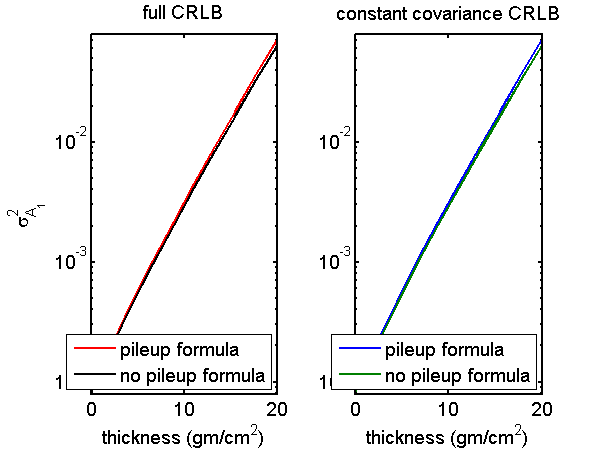
Figure 1 Compare A1 variance computed with no-pileup and pileup formulas. The plot shows the variance on a line through A-space as a function of the distance from the origin. The left plot compares the full variance while the right plot is for the constant covariance approximation. The pileup formulas with zero dead time using the first difference approximations of Eqs. 6↑ and 7↑ are compared with the actual derivatives in Eqs. 4↑ and 5↑.
Constant covariance CRLB error with pileup
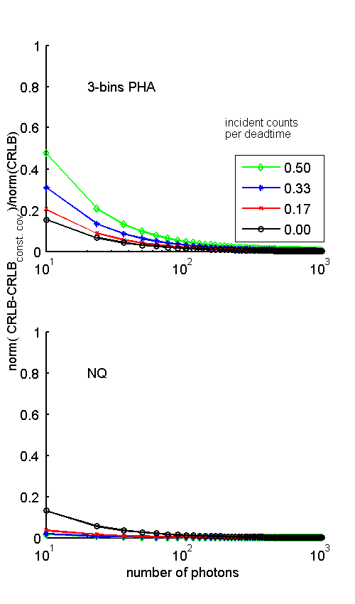
We can define the fractional error as
(8) frac.err. = (∥CA, CRLB − CA, CRLB, const cov∥)/(∥CA, CRLB∥)
where the symbol ∥ ∥ denotes a matrix norm. Fig. 2↓ shows the error as a function of the number of photons for five values of the pileup parameter, η photons per dead time. The top plot is for three bin PHA and the bottom is for the NQ detector. Notice that for a given number of photons, the error with PHA increases but the error with the NQ detector decreases as η increases.
Conclusion
Both with and without pileup, the constant covariance approximation to the CRLB is accurate for photon counts less than those used in material selective applications.
--Bob Alvarez
Last edited Feb 01, 2015
Copyright © 2015 by Robert E. Alvarez
Linking is allowed but reposting or mirroring is expressly forbidden.
References
[1] : “Signal to noise ratio of energy selective x-ray photon counting systems with pileup”, Med. Phys., pp. -, 2014.
[2] : “Dimensionality and noise in energy selective x-ray imaging”, Medical physics, pp. 111909, 2013.
[3] : Fundamentals of Statistical Signal Processing, Volume I: Estimation Theory . Prentice Hall PTR, 1993.