Detection theory with A-space data

In my last posts I discussed the background for applying statistical detection theory to x-ray imaging. In this post, I will show how to incorporate the A-space description into the model. This will lead me to discuss the effect of the basis set functions on the approximation or representation error of the attenuation coefficients of body materials. I will show that there are optimal functions that minimize the error but that other basis functions, such as the attenuation coefficient functions of different materials, do not lead to substantially larger errors. Once the A-space description is in the model, we can derive a signal to noise ratio that is directly comparable to the Tapiovaara-Wagner SNR[3] and we can compare the SNR with limited energy resolution to the ideal with complete spectral information.

Detection theory with the two function basis set

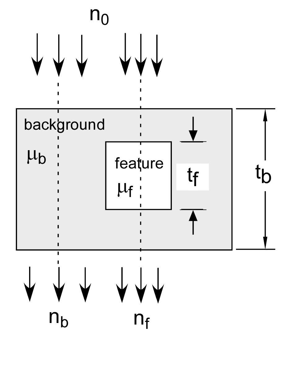
Tapiovaara and Wagner analyzed detecting an object based on measurements of the transmitted spectra as shown in Fig. 1↓. The object consists of a feature with attenuation coefficient μ_f(E) and thickness t_f and a background material μ_b(E) with thickness t_b. We can introduce the A-space description into the analysis by using μ_f(E) and μ_b(E) as the basis functions. Early on in the development of the A-space approach I realized that the attenuation coefficients of any two distinct materials can be used as the basis set (see Sec. 4.5 of my dissertation and my 1979 paper[1]). This is easy to see because the A-space approach converts the attenuation coefficient to a two-dimensional vector and, in a 2D space, any two non-collinear vectors can be used as a basis. However, μ-space is not exactly two dimensional and any two function basis set will have a fit error to the actual data. The error depends on the basis functions so I will discuss this further in the next section.

Figure 1 The Tapiovaara-Wagner imaging task.

With the μ_f(E) and μ_b(E) basis set, the a vectors for the feature and background materials are simply

a_f = ⎡⎢⎣ 1 0 ⎤⎥⎦, a_b = ⎡⎢⎣ 0 1 ⎤⎥⎦.

The A-vector in the background region is A_b = t_ba_b while in the feature region it is A_f = (t_b − t_f)a_b + t_fa_f . We can apply the statistical detection theory model described in my last post by assuming that the A-vector data are described by a multinormal distribution with expected values under two hypotheses: ⟨A_H0⟩ = A_b and ⟨A_H1⟩ = A_f and a covariance C_A. From my last post, the performance will depend only on the signal to noise ratio

(1) SNR² = δA^TC^− 1_AδA

where δA = ⟨A_H1⟩ − ⟨A_H0⟩.

Material attenuation vs. optimal basis functions

The physical material basis set is often used in implementations because the A-vectors for a calibration phantom are the thicknesses of the two materials, which can be measured easily and precisely. For calibration, we usually pick materials with atomic numbers spanning those found in the object such as aluminum and acrylic plastic for biological materials. In the detection theory analysis, however, we may have materials with similar composition. Therefore, we need to study how the approximation error depends on the basis functions.

A first question is whether there is an ideal set of functions. The answer is yes and they are provided by the singular value decomposition (SVD). Recall from my discussion that the SVD expands any matrix B as

B = UDV^T

where I have assumed that the matrix is real. The matrices U and V are unitary and D is a diagonal matrix. In my previous post I described a theorem that gives the optimal basis functions from the SVD. Suppose we arrange the columns and rows of the unitary matrices U and V so that the values on the diagonal of D are in descending order and that we set all the diagonal elements in D for rows greater than r + 1 equal to zero. That is let D_a = diag(σ₁, σ₂, …, σ_r, 0, …, 0). Then Theorem 6.7 of Stewart[2] shows that the matrix B_a = UD_aV^T is the best approximation of B with rank r. That is, the Frobenius norm of the difference ∥B − B_a∥ is the minimum over all matrices of rank r. By this construction, we are selecting the first r columns of U as the basis set so they are the optimal functions and the norm ∥B − B_a∥ is the minimum approximation error.

The next question is how the use of the attenuation coefficient functions of materials whose atomic numbers are close affects the approximation error. To answer this, I did a simulation using the elements found in body materials. I computed a matrix with the attenuation coefficients of the 13 most common elements in body materials along the columns at 100 energies from 20 to 150 keV along the rows. I fixed one of the basis functions as the attenuation coefficient of hydrogen and then computed the norm of the difference between the least squares fit and the actual data using each of the other elements as the remaining basis function. I normalized the errors by dividing by the error with the optimal basis functions from the SVD of the attenuation coefficient matrix.

The results are shown in Fig. 2↓. The left panel shows the optimal basis functions. These are obviously not physical attenuation coefficients but are the mathematical optimal functions. The right panel shows the normalized error as a function of the atomic number of the second function. There are several aspects of these that are of interest. First, as expected, all the normalized errors are greater than one so the first two columns of the U are indeed optimal. However, the errors for elements from 15 to 19 are quite close to the ideal value. The most important result of the simulation for the use of the background/feature basis set is that the errors are not substantially different over the range of elements. Interestingly the largest errors are at the end of the range but even for these the errors are only about 2.5 times the optimal minimum.

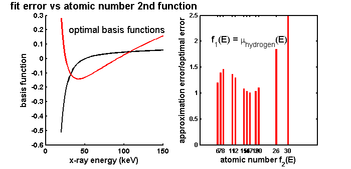
Figure 2 Approximation error with material basis functions versus atomic number spread (right panel). The error is the norm of the difference of the values estimated with a two function basis set and the actual values. The error is relatively constant even if the difference in the materials’ atomic numbers is not large. The errors are normalized by dividing by the error with the optimal set of basis functions, which are the two eigenfunctions of the covariance with the largest eigenvalues. These are plotted in the left panel.

Conclusions

My conclusion is that we can use the background/feature set in our analysis without substantially affecting the results. The next step is to derive the covariance of the A-vector data C_A in the equation for the SNR² (1↑). This depends on the covariance of the logarithm of the x-ray data L and the relationship will require us to use statistical estimation theory as I will describe in my next post.

--Bob Alvarez

Last edited Jan 24, 2012

Linking is allowed but reposting or mirroring is expressly forbidden.

References

[1] Robert E Alvarez, Edward J Seppi: “A comparison of noise and dose in conventional and energy selective computed tomography”, IEEE_J_NS, pp. 2853—2856, 1979.

[2] G. W. Stewart: Introduction to Matrix Computations. Academic Press, 1973.

[3] M. J. Tapiovaara, R. Wagner: “SNR and DQE analysis of broad spectrum X-ray imaging”, Phys. Med. Biol., pp. 519—529, 1985.