If you have trouble viewing this, try the pdf of this post.

An improved parallel projection image reconstructor for Matlab

This post describes a replacement for iradon for Matlab and Octave. The new function, CTrecon.m,

Fixes a bug in iradon that results in offsets from the true values in the reconstructed image.
Uses a mex function from iradon_speedy for backprojection. According to a comment by Jeff Orchard, the author of iradon_speedy, on the Mathworks File Exchange entry for iradon_speedy, Matlab R2011a now uses a mex function. I do not have that version so I cannot confirm this.
Handles complex projections to return a complex reconstructed image - see zBackproject.c
Regularizes the interface to (parameter − name’, parameter − value) syntax. This implies that CTrecon cannot just be dropped in for iradon. The advantage is more readable code.

Another difference is that CTrecon only implements the nearest-neighbor and linear interpolation methods in the backprojection. I have never used the other methods in iradon but if you need them you can extend the C code.

The offset bug is introduced during the calculation of the convolution function. The iradon function uses the convolution-backprojection algorithm[1]. As the name implies, this algorithm first convolves the projections and then back projects them onto the image pixels. With continuous, i.e. non-digitized, functions the transfer function of the convolution is just the absolute value of frequency |w|. The iradon code (see the listing below) discretizes this by using the absolute value of the frequency samples. This is not what we want to do and leads to inaccuracies in the value of the reconstructed image. The problem with this occurs mainly at the zero frequency value. As discussed by Kak and Slaney[1], with a finite bandwidth sampled system, this zeros out the contribution not only at zero frequency but for the complete interval around zero.

To fix the problem, Kak and Slaney suggest computing the convolution function by transforming a discrete version based on a finite bandwidth transfer function (see Eq. 61 in Ch. 3 of their book).

h(nτ) = ⎧⎪⎨⎪⎩ 1 ⁄ 4τ² n = 0 0 n even − 1 ⁄ (Π²n²τ²) n odd

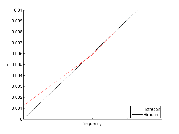
where τ is the distance between projection lines. This is the method used in CTrecon (see the second code box). Fig. 1↓ is a plot of the transfer function near the origin. Notice that the value of the CTrecon transfer function is not equal to 0 at 0 frequency. It is interesting that the Matlab documentation for iradon references the Kak and Slaney book but they do not use their suggested implementation.

             % iradon code
% First create a ramp filter - go up to the next highest power of 2. 
order = max(64,2^nextpow2(2*len));
filt = 2*( 0:(order/2) )./order; % this is the filter spectrum

The problem is illustrated with the simple object shown in Fig. 2↓. The white region has a value 1 and the dark is 0. Suppose we reconstruct using iradon and plot the results. Fig. 3↓ shows the image data along a horizontal line through the center of the five circles. Notice that the values are offset from 0 and 1. Fig. 4↓ shows the reconstruction with CTrecon. The reconstructed values now go through 0 and 1. The ripples on the data are caused by aliasing artifacts since we have a sampled data system.

            % CTrecon code
% create filter by transforming the direct space formula
% (Eq. 61 of Kak and Slaney)
                % the filter order is the next highest power of 2.
order = max(64,2^nextpow2(2*nlines));
filt_length = numel( 0:(order/2) );
ns = 0:(filt_length-1);
h = zeros(size(ns));
h(1) = 0.25;
h(ns(2:2:end)+1) = (-1/pi^2)./ns(2:2:end).^2;
h = [h ,  h(end-1:-1:2)]; % make into form for circular convolve
filt_all = fft(h);

Figure 1 Plot of iradon and CTrecon transfer function.

You may say that the offsets are not very large but one of the principal advantages of computed tomography (CT) is its numerical accuracy. The numerical values in the lungs are used, for example, by radiologists to distinguish between normal lungs and those with emphysema. The Hounsfield unit (HU) is

HU = 1000(μ − μ_water)/(μ_water)

and a 1% difference i.e. 10 HU is considered significant.

As discussed in my previous post, the attenuation as a function of energy is determined by a low dimension vector, length 2 for ordinary body materials and length 3 if there is an externally administered contrast agent present. In the body material case, we can utilize the tight integration of complex numbers into Matlab to represent the attenuation as a complex number. The reconstructed image is then a complex array with the real part equal to the first component and the imaginary part the second. The Matlab functions handle complex data seamlessly so all the filtering operations in CTrecon using fft and ifft do not require any changes. I extended the Backproject.c function for complex data in zBackproject.c, which is used by CTrecon if the projection data are complex.

Finally, I find the calling convention of iradon with a variable number of unlabeled parameters confusing so I adopted the ’parameter − name’, parameter − value calling syntax, which is used by some Matlab functions. See the help for CTrecon for the parameters and their labels.

And, as Steve Jobs says, “one more thing.” The projection data in Fig. 2↓ were NOT computed using the radon function. This function uses a discrete image as its input and leads to large artifacts in the reconstructed images due to ripple when the projection lines align with the rows and columns of pixels in the image. My next post shows an alternate method to compute projections that is more suitable for quantitative work.

You can download code for CTrecon.m and to compute the results in this post here. To use the code, unzip the file into a directory. Compile the C files using mex. See the Matlab help for the mex function for instructions. I find that changing the working directory to the directory with the code using cd makes the compilation much simpler. I have tested the code with the free Microsoft Visual Studio Express 2008 compiler.

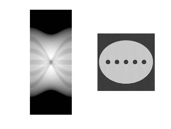
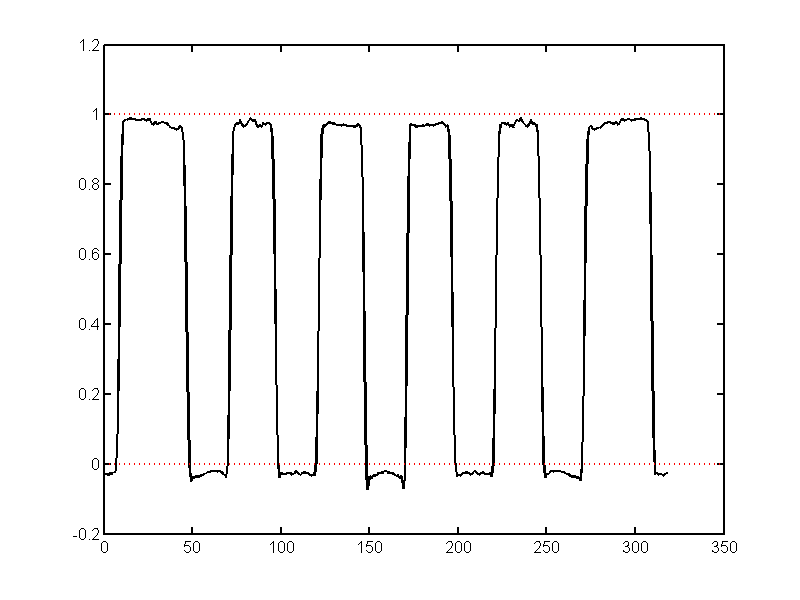
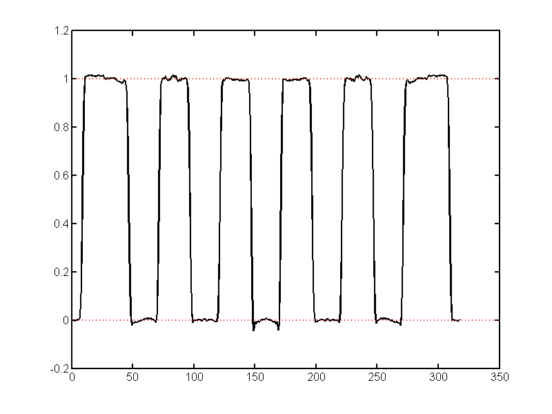
Figure 2 The object projections and the reconstructed image. The projections are in the left panel while the object is on the right. The white values in the object have a value of 1 and the dark a value of 0.

Figure 3 A plot of the data on a line through the center of the iradon reconstructed image. Note the offsets of the data from the true values of 0 and 1. The ripples are caused by aliasing artifacts, which are present in any sampled data system.

Figure 4 Plot of the CTrecon reconstructed image data on the same line used with Fig. 3↑. Note the the data do not show an offset.

Last edited Aug. 7, 2011 to add plot of transfer functions.

Linking is allowed but reposting or mirroring is expressly forbidden.

References

[1] Avinash C. Kak, Malcolm Slaney: Principles of Computerized Tomographic Imaging. Society for Industrial Mathematics, 2001. URL http://www.slaney.org/pct/.