Estimator for contrast agents 1

The next series of posts discuss my recently published paper[2], “Efficient, non-iterative estimator for imaging contrast agents with spectral x-ray detectors,” available for free download here. The paper extends the previous A-table estimator[1], see this post, to three or more dimension basis sets so it can be used with high atomic number contrast agents. It also compares the A-table estimator to an iterative estimator.

This post describes the software to implement the new estimator. The next posts describe the code for an iterative estimator, compare the performance of the new estimator to the iterative estimator and the CRLB, compare the new estimator with a neural network estimator, and finally discuss an alternate implementation using a neural network as the interpolator.

The A-table estimator for higher dimension A-vectors

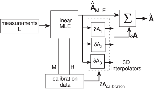
A block diagram of the estimator for three dimensions is shown in Fig. 1↓. I will discuss the main differences between the two and three dimension estimators in the linear maximum likelihood estimator (MLE), the calibrator and the error interpolator.

Figure 1 Block diagram of three dimension A-table estimator.

The linear maximum likelihood estimator

With matrix notation, the form of the linear MLE does not change although the dimensions of the matrices are different.

(1) Â_MLE = [(M^TC^− 1_LM)^− 1 M^TC^− 1_L]L

The equation assumes a linear model with multivariate normal noise:

δL = MδA + w

where A is the vector of the line integrals of the basis set coefficients, L is the vector of the negative logarithm of the measurements for each spectrum divided by the “air” value, M = ^∂L⁄_∂A where the division means that corresponding elements of the vectors are divided, and w is a zero mean multivariate normal random vector with covariance C_L.

The linear estimator is the term in brackets of Eq. 1↑ and is a matrix so the estimates are computed as a matrix multiplication. See the paper and my blog post for a discussion of why we can use a single constant estimator despite the fact that C_L depends strongly on A.

We can compute the parameters required for the estimator from the calibrator data by extending the method for the 2D estimator described in this post. The Matlab code to do this, from AtableSolveEquations3.m, which is included with the code for this post, is

 % solve for M matrix from calibration data
     M = (cdat.As\cdat.logI)’; % note transpose
       % compute MLE inverse solution matrix from M and the covariance
     RLi = inv(cdat.RL);
     cslin = inv(M’*RLi*M)*M’*RLi;
     As_MLE_calibrator = cdat.logI*(cslin’);

It is a straightforward implementation of the expression in brackets in Eq. 1↑. In the code, cdat is the calibration data structure with fields cdat.As i, the thicknesses of the steps of the calibrator arranged on the rows, cdat.logI, the negative of the logarithm of the measurements divided by the measurements with a zero thickness object, L in Eq. 1↑, and finally RL, the covariance of the L on a calibrator step in the middle of the range of A-vectors spanned by the calibrator.

The code computes M as the least squares fit of L as a function of the A with the calibrator data. In Matlab the backslash operator does the least squares fit. Recall that for for linear model, M = ^∂L⁄_∂A so by fitting the data we get an average value over the calibrator data. The next step computes the inverse of the covariance matrix C_L, which is called RL in the code.The next line implements Eq. 1↑ to compute the linear MLE in the brackets of the equation. The final line computes the linear maximum likelihood estimates of the calibrator data.

The 3D calibrator

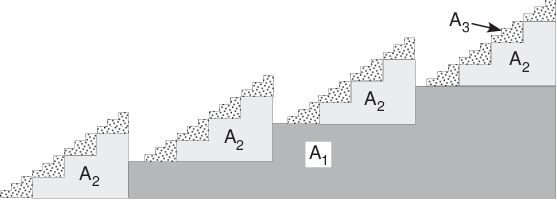
We can extend the 2D calibrator by adding step wedges of the a third basis material. With a contrast agent, the third material might be a machinable plastic material with the high atomic number atoms linked into it so they are uniformly dispersed. A side view of the calibrator is shown in Fig. 2↓. In practice, the step wedges would have more steps. As the number of steps increases, the total number of combinations increases as the cube of the number of steps, so an automated method to make the measurements would be desirable.

Figure 2 Calibrator for a three dimension basis set.

The 3D error interpolator

The implementation of the estimator in my previous paper[1] used the Matlab gridfit.m function[3], which is inherently two dimensional. In order to use the estimator with higher dimension basis sets, we need to find a new interpolator bearing in mind that it needs to operate with non-regularly spaced data. I chose to use the scatteredInterpolant object although other algorithms are certainly possible. A possibility is to use a neural network, which is discussed in a future post.

The error interpolator is constructed by the following code in AtableSolveEquations3.m

              % compute the error vectors for the interpolation
     As_errors_calibrator =  cdat.As - As_MLE_calibrator;
     % errors at uneven spaced As_MLE_calibrator, 
     % ncalibrator_steps by nbasis matrix
     
      % compute the Delaunay simplices 
      % using the first component of As_errors_calibrator as Values
      % since scatteredInterpolant only interpolates scalar data
      % then will make copies of object to duplicate the simplices
      % but use as Values the other 2 components of As_errors_calibrator
      % saves some time with large number of calibration points
     interps = cell(3,1); % this will hold the scatteredInterpolant objects
         % use default linear interpolation and extrapolation methods
      interps{1} = ...
        scatteredInterpolant(As_MLE_calibrator,As_errors_calibrator(:,1)); 
     for kbasis = 2:nbasis
         % make copy of object with its simplices
        interps{kbasis} = interps{1};
          % but substititute data for other components of As_errors_calibrator
        interps{kbasis}.Values = As_errors_calibrator(:,kbasis);
     end

The first line computes the error correction vectors as the differences between the actual calibrator step wedge thicknesses and the linear maximum likelihood estimates. The next lines compute the scatteredInterpolant objects for each dimension of the data. The Matlab scatteredInterpolant object encapsulates the Delaunay simplices, the scalar interpolant data, and the code to compute the interpolated value of a given input data point as a linear combination of the values of the interpolants at the vertices of the enclosing simplex multiplied by the barycentric coordinates. The interpolant data are loaded into the Values member of the object automatically when it is constructed or other data can be substituted after construction. See the comments in the code for a more detailed explanation of its functioning.

Compute the estimates during image acquisition

The following code computes the estimates. The object data are in the tdat structure. The parameters to do the computation such as the Delaunay simplices are stored in the solvedat structure. This is computed once when the AtableSolveEquations3.m is first called but after that, it can be passed as a parameter to the function thus speeding up the computation.

  % linear maximum likelihood estimates for object
As_MLE_object = tdat.logI*(solvedat.cslin)’;
       % solve for correction vectors for the As_MLE_object
As_errors_object = zeros(size(As_MLE_object)); % pre-allocate matrix

for kbasis = 1:nbasis
    As_errors_object(:,kbasis) = solvedat.interps{kbasis}(As_MLE_object);
end

    % add As_errors_object to AsMLE to get final estimate
Astest = As_MLE_object + As_errors_object;

The first line computes the linear maximum likelihood estimates using Eq. 1↑ with the parameters stored in solvedat.cslin. The next lines compute the correction vectors for these estimates and the last line computes the final estimates as the linear maximum likelihood estimates plus the corrections.

Discussion

There are significant differences between the scatteredInterpolant and gridfit interpolators. John D’errico, the creator of gridfit says that it is not an interpolator but an approximator. It fits a two dimensional plate to the data with rigidity constraints so it acts as a smoother. On the other hand, the interpolator in scatteredInterpolant passes through the data points and does a linear interpolation between them. I found that as a result of this I had to use more calibrator steps with the 3D estimator than with the 2D implementation to achieve a negligible bias. There may be alternate interpolators such as a neural network that require fewer steps.

As has unfortunately become increasingly common, Mathworks, Inc., the producer of Matlab, hides the code for the scatteredInterpolant class. In the paper, open source functions that should be able to reproduce the results of the paper and of the posts on the new estimator are described.

Last edited Mar 03, 2016

Linking is allowed but reposting or mirroring is expressly forbidden.

References

[1] Robert E. Alvarez: “Estimator for photon counting energy selective x-ray imaging with multi-bin pulse height analysis”, Med. Phys., pp. 2324—2334, 2011. URL http://www.ncbi.nlm.nih.gov/pubmed/21776766.

[2] Robert E Alvarez: “Efficient, non-iterative estimator for imaging contrast agents with spectral x-ray detectors”, IEEE Trans. Med. Imag., 2015. URL http://dx.doi.org/10.1109/TMI.2015.2510869.

[3] John D'errico: Surface Fitting using gridfit. URL MATLAB Central File Exchange, http://www.mathworks.com/matlabcentral/fileexchange/8998),.