If you have trouble viewing this, try the pdf of this post. You can download the code used to produce the figures in this post.
Beam hardening 4: consistency
In the posts on beam hardening, I have shown that it causes the estimate of the line integral using the single average energy assumption to be nonlinearly related to the actual line integral. The nonlinearity causes any noncircularly symmetric object to look different when you look at it from different angles. This inconsistency results in artifacts in the reconstructed images. That is, the reconstructed image has features in it that are not in the original object. The inconsistency brings up some interesting questions. Is there a way to test the data to determine whether it is inconsistent? If so, is there a way to subtract the inconsistent part and will the result be equal to the original object without artifacts? In this post, I will review some prior research into this subject.
Consistency conditions—the constant projection sum condition
There are two related consistency conditions that have been developed. The first, the constant projection sum condition, is simple to understand yet quite powerful. By the definition of a line integral, we can see that the sum or integral of the line integrals in any direction is equal to the volume of the object in the 3D view. Therefore, if the line integrals are consistent, the sum should be a constant independent of the view angle.
Fig. 1↓ is an example. The top plot is a 3D view of an object with its attenuation coefficient. In this view, the x-y axes are the cross-section coordinates of the slice of the object and the z-axis is the linear attenuation coefficient. The two boxes are cubes so the objects are squares in the cross section of side 1 and they have attenuation coefficients equal to 1. In the case of the figure, the sum of the volume of the boxes is equal to 2.
The middle and bottom plots show the line integrals and their squares for lines parallel to the x and y coordinates respectively. In the middle panel, for lines parallel to the x-axis, the objects do not overlap so the projections and their squares are all equal to 1 and the integral is equal to 2. In the bottom panel, for lines parallel to the y-axis, the boxes overlap. In this case the line integrals are equal to 2 so their square is equal to 4 as shown. In this case the sum of the linear line integrals is again equal to 2 but the sum of the squares is equal to 4. As expected, the squares of the line integrals fail the constant projection sum condition.
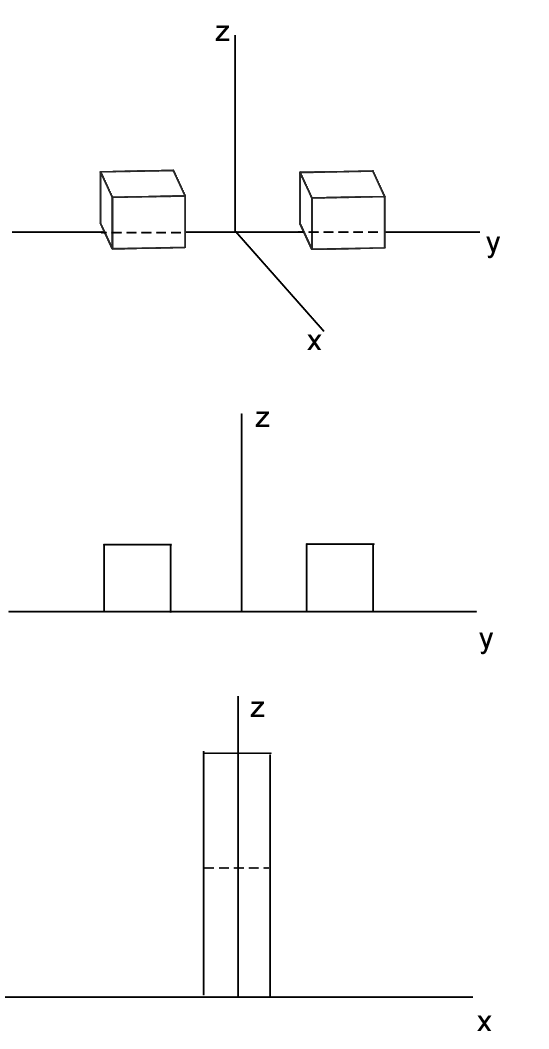
Figure 1 A 3D view of an object in a CT image. The x-y axes are the cross-section coordinates of the slice of the object and the z-axis is the linear attenuation coefficient. The two boxes are cubes so the objects are squares in the cross section of side 1 and they have attenuation coefficients equal to 1.
The moments of the circular harmonic modulator condition
Cormack[2] was probably the first to derive this condition although it has been discussed by many papers. The derivation of the condition is pretty complex so I refer interested readers to Cormack’s paper. The condition is stated in the proof of section 3.f on the sign changes of the radial modulators of the Fourier series of the projection.
The proof starts from the observation that the line integrals f(p) for a given distance p of the line from the origin are a function of angle φ and are periodic with period 2π. In Cormack’s formulation the radii are non-negative, the object is zero outside of radius 1, and the angles go from 0 to 2π. Under some very general mathematical conditions that are always met in practice, we can therefore express them as Fourier series whose coefficients are a function of p.
f(p, φ) = + ∞⎲⎳n = − ∞fn(p)einφ
Similarly, we can decompose any 2D object g(r, θ) as a Fourier series whose coefficients depend on r
g(r, θ) = + ∞⎲⎳n = − ∞gn(r)einθ.
Cormack shows that with the Fourier series the problem separates so for any order n the radial modulators of the projections depend only on the corresponding radial modulators of the object. The two are related by an integral equation
fn(p) = 21⌠⌡p(gn(r)Tn(p ⁄ r)rdr)/((r2 − p2)1⁄2)
where the Tn are Chebyshev polynomials. From the properties of this series of orthogonal polynomials, Cormack showed that the radial modulators of the projections satisfy the following moment conditions
(1) 1⌠⌡0fn(p)pkdp = 0, k < n.
Recall that Cormack assumes that the object is zero for radii greater than one, which is true in all practical cases by properly normalizing the coordinates.
We can use the moment condition to derive the constant projection sum condition but not vice-versa[3].
Does nonlinearity always lead to inconsistency
Ein-Gal[4] suggested that the moment condition be used to remove the “inconsistent” portion of the projections. This raises the question whether nonlinear projections always fail the moment test. A simple counter example shows this is not true. If the object is circularly symmetric then its squared projections still satisfy the moment condition[3]. Although no real object is perfectly circularly symmetric, the closer the object is to having this symmetry the less the utility of the moment condition.
Practical implications of consistency conditions
How often is the moment condition useful? In her article, Patch[5] states
Projecting axial computed tomography (CT) data on to the range of the Radon transform does not improve image quality . However, by monitoring the degree to which CT data satisfies the Helgason-Ludwig range conditions it may be possible to detect failing equipment before serious image artifacts are noticeable.
Helgason-Ludwig are the authors that Patch gives credit for Cormack’s moment condition.
This has also been my experience. The moment conditions, although mathematically elegant, do not provide any substantial reduction in artifacts. The best way to reduce these artifacts is to use my method of solving for the line integrals of the basis set coefficients from multiple spectrum measurements[1]. Next to this method, the physically based methods of pre-filtering and linearization of the line integrals also reduce artifacts but with the limitations that I have discussed in this series of posts.
Conclusion
This concludes my series on beam hardening artifacts. Although they have a long history in CT, they are still a serious problem resulting in quantitative errors that are poorly understood and taken into account by clinical users. They also cause streak artifacts from highly attenuation objects that are a serious problem in head scans of people with metallic tooth fillings and people with artificial joint replacements or other metallic objects in their bodies.
Last edited Sep 10, 2015
Copyright © 2015 by Robert E. Alvarez
Linking is allowed but reposting or mirroring is expressly forbidden.
References
[1] : “Energy-selective reconstructions in X-ray computerized tomography”, Phys. Med. Biol., pp. 733—44, 1976.
[2] : “Representation of a Function by Its Line Integrals, with Some Radiological Applications”, Journal of Applied Physics, pp. 2722—2727, 1963.
[3] : Image Statistics And Nonlinear Artifacts In Computed Transmission X-Ray Tomography. 1979.
[4] : “The shadow transform: An approach to cross sectional imaging”, NASA STI/Recon Technical Report N, pp. 22706, 1974.
[5] : “Moment Conditions Indirectly Improve Image Quality”, Contemporary Mathematics, pp. 193-205, 2000.