Monte Carlo validation of variance formulas

My “SNR with pileup ...” paper[1] presented a set of theoretical formulas for the noise of NQ and PHA detectors in Tables I and II. I have discussed the individual formulas and Monte Carlo simulations of their validity in past posts in this series. In Section 2.K of the paper, I presented an overall test of the formulas that compared the A-vector component variances with a Monte Carlo simulation of the random detector data processed with a maximum likelihood estimator (MLE). In this post, I expand the discussion in the paper and present code to reproduce Fig. 2.

The approach

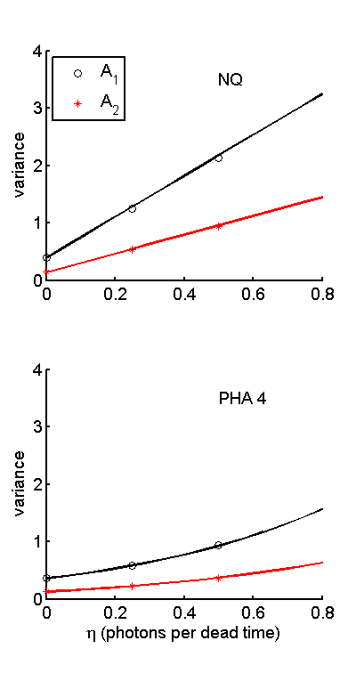
Fig. 2 plots the A-vector variances as a function of the number of photons incident on the detector for three values of η. The theoretical A-vector components noise variances were taken from the diagonal elements of the Cramèr-Rao lower bound (CRLB) computed with the functions CRLB_NQ_with_pileup.m and CRLB_PHA_with_pileup.m. These functions are “cleaned up” versions of the functions used in previous posts in this series. They use the first difference approach to computing the CRLB with pileup described in this post.

The theoretical variances were compared with the sample variances of a set of A-vector values computed from random samples of detector data. The code to generate the random samples of NQ and PHA data is shown in the text box. It is the same as used in a previous post.

1for ktrial = 1:nMCtrials
2    dt_pulse = -(1/mean_cps)*log(rand(npulses2gen,1)); 
3        % exponentially distributed interpulse times
4    [npulses_record, egys_rec] = ...
5        PileupPulses(dt_pulse,deadtime, t_integrate,’specinv’,spinv);
6    nqdat(ktrial, :) = [npulses_record(1), sum(egys_rec)]; 
7        % PHA data
8    counts = histc(egys_rec,egy_bin_edges);
9    phadat(ktrial,:) = counts(1:(end-1));
10end

The next step is to calculate A-vectors from the random data with a linear MLE. The linear MLE, discussed in this post, is

Â_MLE = [(M^TC^− 1_LM)^− 1 M^TC^− 1_L]L

Comparing this with the constant covariance approximation to the CRLB, discussed in this post,

CRLB_{const − cov} = [MC^− 1_LM]^− 1,

we can see that the linear estimator is

Â_MLE = [CRLB_{const − cov}M^TC^− 1_L]L.

This is the formula implemented in the code.

1   % compute linear MLE for NQ and PHA
2[~, nqstats] = CRLB_NQ_with_pileup(specdat,eta);
3MLE_NQ = nqstats.CRLB_const_cov*nqstats.M’*nqstats.RLinv;
4[~, phastats] = CRLB_PHA_with_pileup(specdat,eta);
5MLE_PHA = phastats.CRLB_const_cov*phastats.M’*phastats.RLinv;

The MLE were then applied to the logarithm of the random detector data as as shown in the following text boxes for the NQ detector. The L data are the negative of the logarithm of the measurements divided by the measurements with no object. For the NQ detector, these “air” values are as as shown. Note that the expected value of Q is ⟨Q⟩ = ⟨N⟩⟨E⟩

1LsNQ = -bsxfun(@minus,log(nqdat),log([nphotons, nphotons*Ebar]));
2As_NQ_calc = (MLE_NQ*LsNQ’)’; % use transposes since MLE expects column vector of data

Finally, the bootstrap algorithm was used to compute the mean value and the standard deviation of the mean. The standard deviation can be used to display error bars on the Monte Carlo data, although this was not done in the example since they were too small to display.

1bootstatNQ = bootstrp(nbootstrap,@(x) ToRow(cov(x)),As_NQ_calc);
2RA_NQ_mc = reshape(mean(bootstatNQ),2,2);
3RA_NQ_mc_se = reshape(std(bootstatNQ),2,2);
4RA_NQ_all(:,:,keta,kt) = RA_NQ_mc;
5RA_NQ_all_se(:,:,keta,kt) = RA_NQ_mc_se;
6CRLB_NQ_all(:,:,keta,kt) = nqstats.CRLB;

The PHA results were computed with the same approach.

The plots

The Monte Carlo and theoretical data were plotted by the code in the post code file. The results are shown in Fig. 1↓ for the variances vs. the number of photons and in Fig. 2↓ for the variance at fixed number of photons vs η.

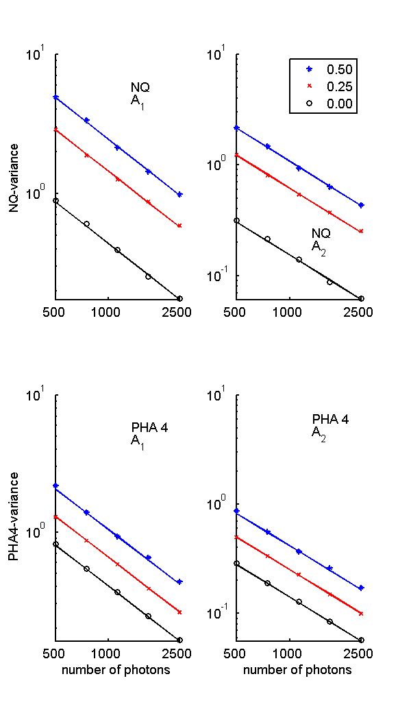
Figure 1 Theoretical and Monte Carlo sample variances. The top panel shows the NQ results and the bottom panel the PHA results. The variances are plotted as a function of the number of photons for three values of η, 0, 0.25 and 0.5. The lines are the theoretical values and the individual symbols are the Monte Carlo sample variances.

Figure 2 Variance as a function of η for fixed number of photons. The top panel is for the NQ and the bottom panel for four bin PHA detectors.

Conclusion

The Monte Carlo values in Fig. 1↑ and 2↑ are close to the theoretical formulas. These results validate but, of course, do not mathematically prove the formulas. Notice that the NQ variance increases fractionally more than the four bin PHA as η increases.

Last edited Feb 10, 2015

Linking is allowed but reposting or mirroring is expressly forbidden.

References

[1] Robert E. Alvarez: “Signal to noise ratio of energy selective x-ray photon counting systems with pileup”, Med. Phys., pp. -, 2014.