If you have trouble viewing this, try the pdf of this post. You can download the code used to produce the figures in this post.
SNR with pileup
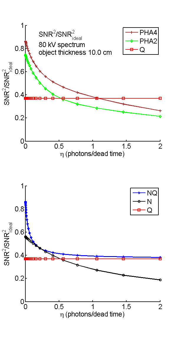
In this post I conclude my discussion of my “SNR with pileup ...” paper[2]. I will present and explain the code to reproduce the “bottom line” figures 3 to 5 of the paper that show the decrease of the SNR as the pileup parameter η increases. The decrease is rapid and when the value of η reaches 1, all the counting and PHA detectors have SNR smaller than the energy integrating detector. The NQ detector SNR decreases rapidly and approaches but marginally stays above the Q SNR since it uses that signal.
The formulas and code
The complete code to compute the SNR for all detector types as a function of η is in cell 4 of the overall code for this post, P53SNRpileup6.m
The parameters required to compute the SNR with pileup are the spectrum incident on the detector and η. The SNR of the ideal, Q, N, and NQ detector are computed by the SNR_with_pileup.m function. The ideal detector SNR was computed using Eq. 36 of my “Near optimal ...” paper[1].
The parameters are explained in the paper: nT(E) is the spectrum transmitted through the object and incident on the detector, tf is the thickness of the feature in the same units as the linear attenuation coefficient μ, δμ(E) is the difference of the basis function attenuation coefficients. The leading term, t2f⁄2 was set equal to one in the code since it is the same for all of the detectors. The ideal SNR was implemented with this code
1dMus = diff(specdat.mus,1,2); % difference along rows
2SNR_ideal = trapz(specdat.egys,specdat.specnum.*(dMus.^2));
The Q detector SNR, from Eq. 34 of the “Near optimal ...” paper[1], is
where the notation
⟨μ(E)⟩Q = ⌠⌡μ(E)q̂(E)dE
means the effective value in the normalized energy spectrum q̂(E). In the equation, λ is the integral of the photon number spectrum, which is the total number of photons, F is the excess variance
F = (⟨E2⟩N)/(⟨E⟩2N)
where the notation ⟨ ⟩N means the effective value of a variable in the normalized photon number spectrum. This was implemented with the following code
1specdat.specegy = specdat.egys.*specdat.specnum;
2specdat.specegy_norm = specdat.specegy/trapz(specdat.egys,specdat.specegy);
3    % SNR of Q (energy integrating) not affected by pileup
4dmusQ = trapz(specdat.egys,specdat.specegy_norm.*dMus);
5SNR_Q = nbar_incident*dmusQ^2/F;
The photon counting N detector SNR used the variance and the M matrix with pileup computed by the NQ detector CRLB function, CRLB_NQ_with_pileup.m. with Eq. 20 of the “Near optimal ...” paper
SNR2N = (ΔA)TMTR − 1LM(ΔA)
where ΔA is the difference of the A-vectors in the background and feature regions. As explained in the “Near optimal ...” paper, by using the attenuation coefficients of the feature and background regions and, since t2f⁄2 was set equal to one in all of the SNR formulas, this was set equal to
ΔA = ⎡⎢⎣
1
− 1
⎤⎥⎦.
For the detectors with pileup, the SNR was computed as
(3) SNR2 = ΔATC − 1AΔA
where CA is the A-vector covariance. The CRLB was used for the covariance since it gives an optimal value that does not depend on the type of estimator. The CRLB functions used the full formula for the Fisher matrix discussed in the last post. Since the Fisher matrix F is the inverse of the CRLB, this was used directly in Eq. 3↑ instead of taking the inverse twice.
The NQ and N detector SNR were implemented with this code
1     % SNR NQ detector
2[~, nqstats] = CRLB_NQ_with_pileup(specdat,eta);
3SNR_NQ = dA’*nqstats.F*dA;
4     % SNR N detector with pileup
5M_N = nqstats.M(1,:); % eff mus for photon count spectrum with pileup
6SNR_N = dA’*M_N’*(1/nqstats.RL(1,1))*M_N*dA; % nqstats.RL is cov of log of NrecQ
The CRLB with PHA was computed by the CRLB_PHA_with_pileup.m function. This function used the idx_threshold field of the spectrum structure, which is the indexes into the egys vector of the PHA bins. This was implemented with the following code from the overall function for this post P53SNRpileup6.m:
1for kbin = 1:nbins2test
2    specdat.idx_threshold = idx_thresholds{kbin};
3    [~,pha_stats] = CRLB_PHA_with_pileup(specdat,eta);
4    SNR_PHA = dA’*(pha_stats.F)*dA; % F is the inverse of the A-vector CRLB
5    ...
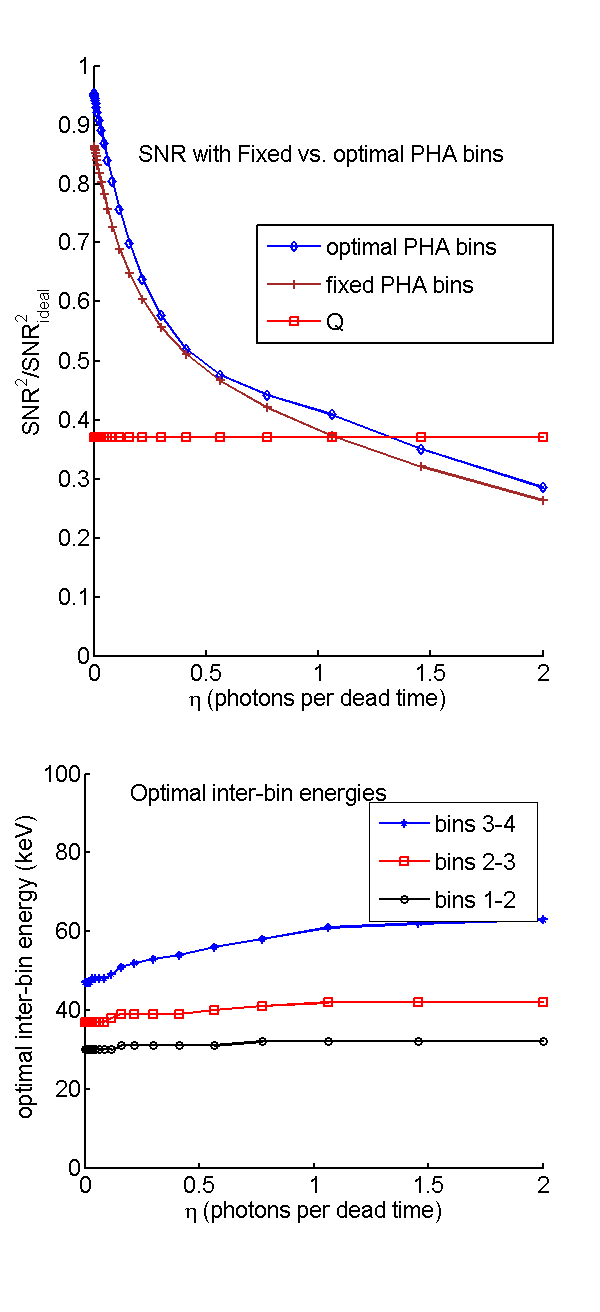
The optimum PHA bins for each value of η are computed by the OptimNbinsThresholdsSNR.m function. This uses a brute force algorithm of computing the SNR for each possible set of bins that span the energy spectrum. Since this rapidly leads to a huge number of combinations the function uses the min_bin_width variable to set the minimum bin. The search is then in two steps: first the optimal bins are computed to within a minimum width, then the combinations around this optimal set are searched. Even with this approach, the computation takes a long time. The code to implement this is in the box
1if get_optimal_bins && (kbin==2)
2        %compute PHA4 SNR with optimal bins with pileup
3    sp_w_pileup = SpectrumWithPileup(specdat,eta);
4         % recompute mus for energies in pileup spectrum
5    sp_w_pileup.mus = MusFromMaterials(materials,sp_w_pileup.egys);
6       % use 2 steps to get optimal bins.
7       % First coarse search
8    [idx_threshold1,Ethreshold1] = OptimNbinsThresholdsSNR(sp_w_pileup,nbins(kbin), ...
9        ’min_bin_width’,2,’dynamic_range’, 100,’verbose’);
10       % then fine search
11   [idx_thresholdSNR,EthresholdSNR] = OptimNbinsThresholdsSNR(sp_w_pileup,nbins(kbin), ...
12        ’min_bin_width’,1,’dynamic_range’, 100, ...
13        ’close_egys’,Ethreshold1,’close_dist’,5,’verbose’);
14    specdat.idx_threshold =  idx_thresholdSNR;
15    [~,pha_stats] = CRLB_PHA_with_pileup(specdat,eta);
16    SNR_PHA_opt = dA’*(pha_stats.F)*dA;
17    SNR_with_deadtime_opt(keta, 4+kbin) = SNR_PHA_opt;
18    Ethreshold_opt = [Ethreshold_opt EthresholdSNR];
19end
Results
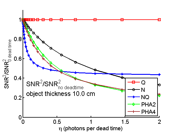
The graphs in Figs. 1↓ and 3↓ should be compared with Figs. 3 and 5 of the paper. Fig. 2↓ was not in the paper but is interesting.
Conclusions
The implications of these results are described in the paper. As discussed in the first post of this series,
The basic assumption that I will make is that these idealized models provide an upper limit to the SNR of real detectors. Obviously, I cannot prove this but it is reasonable to assume that any additional distortions of the data will decrease the SNR. The results will apply to a single measurement so all bets are off if you are, for example, spatially filtering to combine the results from several detectors or making more than one measurement at different times with the same detector and combining the results. Iterative algorithms with “regularity” or smoothness conditions also combine results from different measurements nonlinearly so they will have different SNRs. But in all these cases, having higher quality input data will most likely lead to better final results.
Last edited Feb 09, 2015
Copyright © 2015 by Robert E. Alvarez
Linking is allowed but reposting or mirroring is expressly forbidden.
References
[1] : “Near optimal energy selective x-ray imaging system performance with simple detectors”, Med. Phys., pp. 822—841, 2010.
[2] : “Signal to noise ratio of energy selective x-ray photon counting systems with pileup”, Med. Phys., pp. -, 2014.