If you have trouble viewing this, try the pdf of this post. You can download the code used to produce the figures in this post.
SNR with pileup-4: Probability distribution with pileup
The method to compute SNR in my paper, “Signal to noise ratio of energy selective x-ray photon counting systems with pileup”[1], assumes that the noisy data have a multivariate normal distribution. Appendix A of the paper describes a Monte Carlo simulation to study the conditions under which the normal distribution assumption is valid. In this post, I will expand on the discussion in the paper and present Matlab code to reproduce the figures.
The method
The normal distribution assumption is tested using Royston’s test[2] for multivariate normality. The background and the algorithm for the test are discussed in this post. In this post, the Royston test was applied to show that NQ data without pileup are normally distributed for large enough counts. We cannot simply apply the test to a sample of data since the test results are also random. However, by repeating the tests and averaging the results, we can increase the accuracy of our estimate of the true probability of a normal distribution. For data with pileup, the required counts are also a function of the pileup parameter, η, the expected photons per dead time. Therefore, the simulations were repeated for a range of the parameter values. For each value of η, we can plot the mean values of the Royston test results as a function of the average counts. By fitting a sigmoid function to these plots, we can determine the counts so that the probability that we not reject the normal hypothesis is a specified amount, 0.9 for the computations in the SNR with pileup paper.
The software
The code to generate random data with pileup is in code cell block 4 and is in the text box below. The approach is the same as in the last post. As shown in the text box, the code generates both NQ and PHA data from the same random sample of interphoton times and recorded energies.
1dt_pulse = -(1/mean_cps)*log(rand(npulses2gen,1));
2    % exponentially distributed interpulse times
3[npulses_record, egys_rec] = ...
4    PileupPulses(dt_pulse,deadtime, t_integrate,’specinv’,spinv);
5nqdat(ktrial, :) = [npulses_record(1), sum(egys_rec)];
6    % PHA data
7for kbins_case = 1:nbins_cases
8    counts = histc(egys_rec,egy_bin_edges{kbins_case});
9    phadat(kbins_case, ktrial,1:nbins(kbins_case)) =  ...
10        counts(1:(end-1));
11end
Once a random sample is generated, it used to compute the hypothesis test result for normality using Royston’s test as implemented in the roystest.m function[3]. For the linear data this is straightforward but care must be taken with log data to exclude zero values. With PHA data, the zeros are changed into ones.
1counts_dat(counts_dat(:)==0) = 1;
With the zero counts NQ data, we need to substitute a small number for the recorded energy Q, which is a floating point number. A value equal to 0.001 of the Q expected value is used, where the 0.001 fraction was arbitrarily chosen to have a minimal effect on the results. The bsxfun function was used to promote the number of rows of the substituted values to be the same as the number of zero counts cases.
1nqdat(nqdat(:,1)==0,:) = bsxfun(@plus,nqdat(nqdat(:,1)==0,:), ...
2       [1 0.001*specdat.Ebar*mean_cps*t_integrate]);
The Royston’s test results were stored in the multidimensional array, Hs. To make the code more readable, a Map container object detsmap was used so the results for each type of detector could be accessed by their text description. An example is shown in the text box
1dets = {’NQlin’,’NQlog’,’PHA2lin’,’PHA2log’,’PHA4lin’,’PHA4log’};
2ndets = length(dets);
3detsmap = containers.Map(dets,1:ndets);
4...
5Hs(detsmap(’NQlin’), kdeadtime, kt, krun) = stats_roy.H;
A sigmoid function was fit to the average probability as a function of counts data. By “sigmoid” I mean an S-shaped function that is zero for small counts and one for large counts. You can see examples in Figures 1↓ to 3↓. For ease of computation, I chose a function with a straight line transition from 0 to 1. It was therefore parametrized by the x-values of the end points of the transition region. The Matlab nlinfit function was used to fit the data. The computation was done in code cell 6 during the display of the data. The mean and standard deviation of the Royston test results were computed using the bootstrap method and the average counts from the bootstrap were fit to the sigmoid function. The bootstrap standard deviation was used to compute errorbars for the plotted data
1beta_fit = ...
2nlinfit(nphotons(:),Hs_bar_bootstrap(:),@sigmoid_line,[0 max(nphotons)]);
Results
The probability versus the number photons was computed for different η and different detectors. The results are in Figures 1↓ to 3↓.
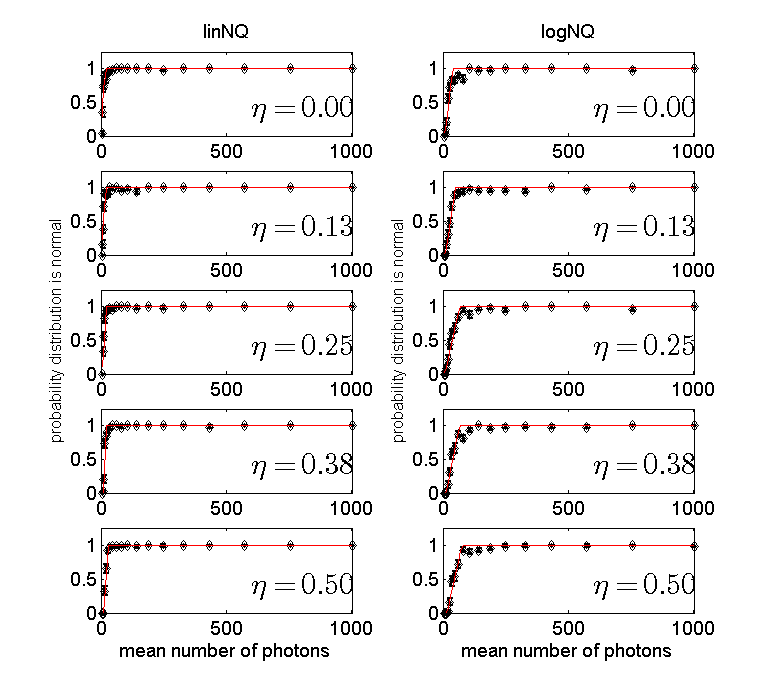
Figure 1 Probability to accept normal model for NQ detector data as a function of the number of photons. The left column is for the NQ data while the right column of for the logarithm of the data. Each row is for a different value of the expected number of photons per dead time parameter, η. The best sigmoid fit function is plotted as the solid lines.
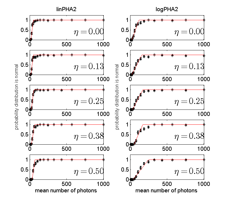
Figure 2 Probability to accept normal model for 2 bin PHA detector data as a function of the number of photons. The left column is for the data while the right column of for the logarithm of the data. Note that more photons are needed to accept the normal model with this detector than with the NQ detector.
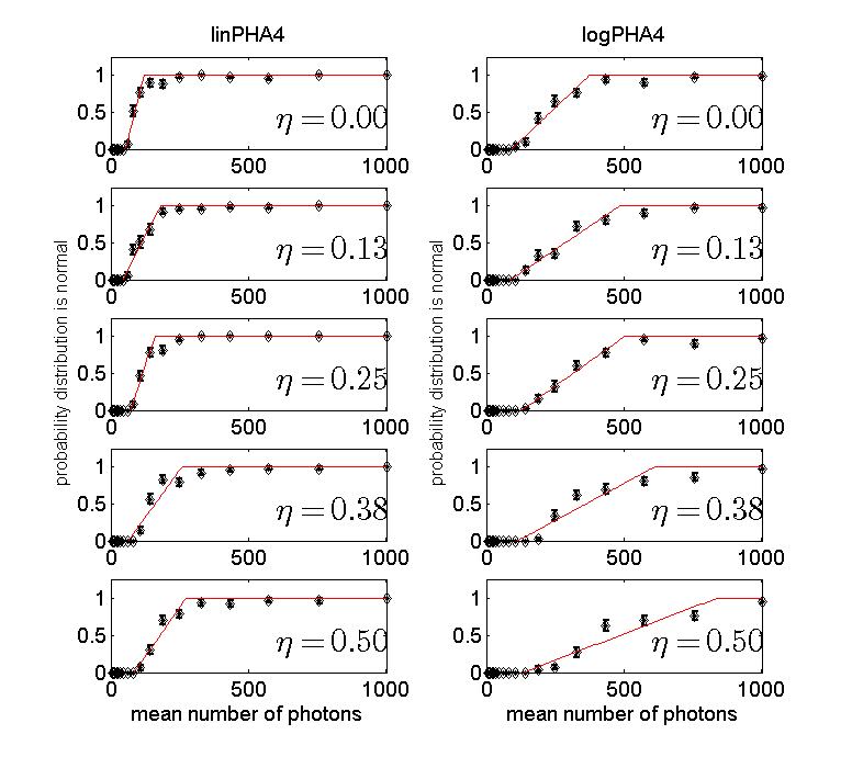
Figure 3 Probability to accept normal model for 4 bin PHA detector data as a function of the number of photons. The left column is for the data while the right column of for the logarithm of the data. More photons are needed with four bin PHA than with two bin and the NQ detector.
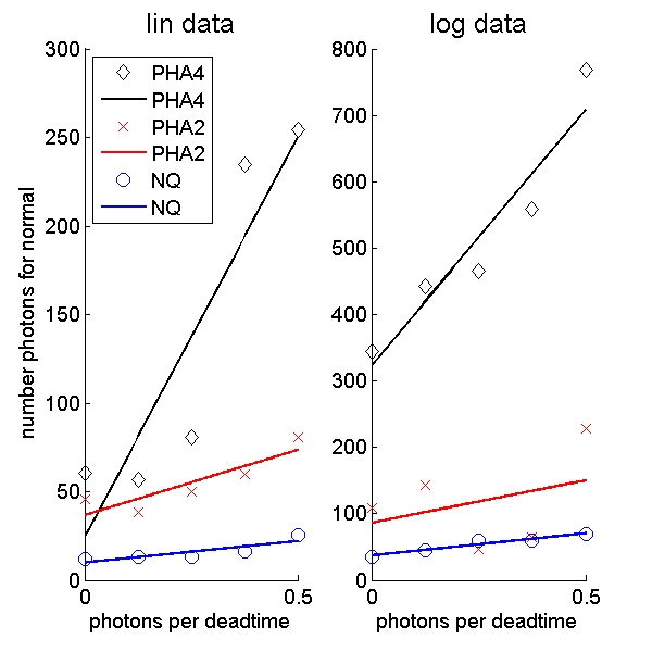
Figure 4 Number of photons for 90 percent probability not to reject the normal model for data from different detector types as a function of the pileup parameter, η. The left plot is for the linear data while the right plot is for the logarithm of the data. The solid lines are a straight line fit to the data.
Conclusion
The probability not to reject the normal model approaches one for large enough number of photons for all detectors. The number of photons required is small compared to those used in material selective imaging.
Bob Alvarez
Last edited Jan 26, 2015
Copyright © 2015 by Robert E. Alvarez
Linking is allowed but reposting or mirroring is expressly forbidden.
References
[1] : “Signal to noise ratio of energy selective x-ray photon counting systems with pileup”, Med. Phys., pp. -, 2014.
[2] : “Some Techniques for Assessing Multivarate Normality Based on the Shapiro- Wilk W”, J. R. Stat. Soc. Ser. C (Appl. Stat.), pp. 121—133, 1983.
[3] : Roystest: Royston's Multivariate Normality Test. A MATLAB file.. URL MATLAB Central File Exchange, http://www.mathworks.com/matlabcentral/fileexchange/17811.