Improve noise by throwing away photons?
Photon counting systems with pulse height analysis (PHA) count the number of photons whose energy falls within a set of energy ranges, which I will call bins. Usually the bins are contiguous, non-overlapping, and span the incident energy spectrum so each photon falls within one bin. A paper
[6] by Wang and Pelc showed that the A-vector noise variance can be decreased by using bins that are not contiguous. That is, if we use bins that only cover the low and high energy regions and do not include intermediate energies, we can lower the noise variance. Photons with energies in these intermediate regions are not counted i.e. they are thrown away. Improving noise by throwing away photons is an interesting concept and I will discuss it in this post. It turns out to be an example where the choice of the quality measure fundamentally changes the hardware design, which happens often, so it is important to study it.
Noise variance--two competing factors
We can understand the rationale for improving noise by throwing away photons from the equations for the Cramèr-Rao lower bound (CRLB) of the noise variance of the A-vector components with photon counting noise (see for example my paper
[1]):
In these equations, ⟨N1⟩ and ⟨N2⟩ are the expected values of the measurements and M is the matrix of the effective basis functions for the two spectra. Notice that the variances depend on two factors: the numerators with 1 ⁄ ⟨N⟩ terms that get larger as the number of photons decrease and the denominator, which is the square of the determinant of M, which gets larger as the “conditioning” of the transformation from the measurements to the A-vector gets better.
Non-contiguous PHA
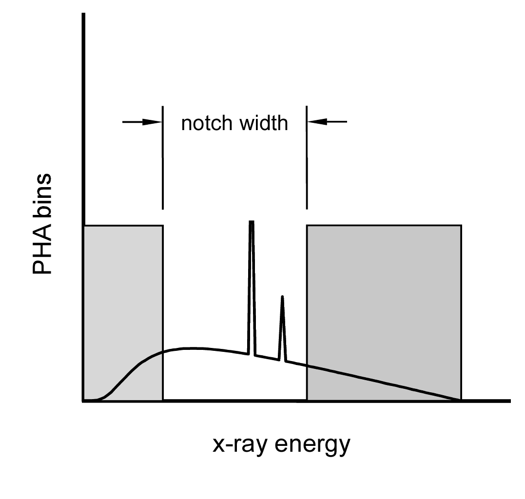
A PHA system with non-contiguous bins is shown in Fig.
1↓. The shaded regions represent the bin response functions and photons with energies in these regions are counted. Photons with energies in the clear area, the notch, are not counted. Since the photons in the center of the energy spectrum tend to reduce the difference in average energies in the bins, we can improve the conditioning of the
M matrix and therefore reduce the noise by throwing away those photons. However, as we increase the notch width, the number of counts
⟨N1⟩ and
⟨N2⟩ decreases and the numerator in equations increases as discussed in the previous section. Depending on the relative size of the two factors, there may be an optimal notch width that gives a minimum variance.
The
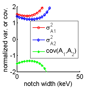
package for this post has Matlab code to compute the variances as a function of notch width. The results are shown in Fig.
2↓. Notice that the variances of both components go through a minimum although they do so at slightly different notch widths.
The results in Fig.
2↑ show that the variances indeed go through a minimum that is lower than the value with contiguous bins. Wang and Pelc show that 3 bin PHA with non-contiguous bins can also result in lower variance.
Noise covariance
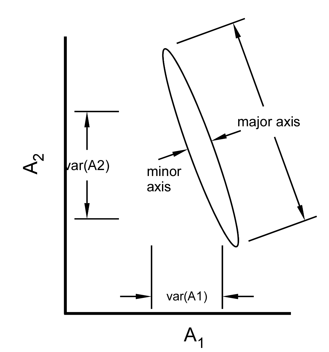
Although variance is important, A-vector noise is highly negatively correlated and is not fully specified by the variances. As shown by Fig.
3↓ the variances can be misleading in some cases. The figure shows a cross section of the two-dimensional probability distribution of A-vector data. I have shown several times (for example
in this post) that the distribution is accurately modeled as multivariate normal so it has elliptical contour curves. Even though the distribution is highly non-isotropic with a large negative correlation, the two variances, which measure the marginal distributions on the
A1 and
A2 axes are nearly equal.
The covariance for the two spectrum case is
This equation was used to compute the covariance in the bottom part of Fig.
3↑. Notice that the covariance has a maximum, that is, it less negative around that same notch width where the variances reach a minimum.
Noise covariance and SNR
One way to quantify the effect of noise is to see how it affects an imaging task, such as detecting the presence of a feature in background material. A method to analyze this was presented in my paper, “
Near optimal energy selective x-ray imaging system performance with simple detectors[5], which was discussed in a series of posts starting with
this one.
In the paper and the posts, I showed that the detection performance depends on the signal to noise ratio (SNR), which for a vector quantity like the A-vector is defined to be
where
δA is the difference in the A-vectors of the feature and background regions of the object and
C − 1A is the inverse of the A-vector covariance. From this equation, it is clear that the SNR depends on the full covariance matrix--not just on the variances of the individual components.
The SNR vs. notch width
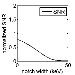
We can use the same simulation software used to produce Fig.
2↑ to compute the SNR as a function of the notch width. The result is in Fig.
4↓. Notice that the SNR always decreases as the notch width increases. The optimal width is zero.
Discussion
The optimal system design depends on the quality measure. If we just display the images of each A-vector component, then we should minimize the noise variance and the results in Fig.
2↑ show that we should use a non-zero notch width where the variances of the A-vector components go through a minimum.
If we use SNR as a quality measure, then we need to use the full covariance as shown in Eq.
4↑. Fig.
2↑ shows that the covariance becomes less negative for notch widths that minimize variance. Combining these, Fig.
4↑ shows that the SNR always decreases as notch width increases even though the variances decrease. As a result, the optimal notch width for the maximum SNR is zero.
Which quality measure to use depends on the end use of the data and is somewhat subjective. I think SNR is a better measure than the variance for most applications. Standard detection theory shows that the error rate in the detection imaging task depends on the SNR. As shown in the discussion of my “Near optimal ...” paper, we can use a linear transformation to create A-vectors with whitened noise that has zero covariance. The noise is easier to interpret in these coordinates and, as shown in Section II.H of the paper, it will have the same SNR as in the original A-vector space.
Covariance is an important part of the noise. Even for the display of the A-vector components, the negative covariance can be used, as shown
in this post, to produce lower noise images. Using PHA with a notch affects the covariance in addition to the variances and may reduce the effectiveness of the correlation noise reduction.
Photon counting with PHA is still not practical for most medical imaging applications so the most common way to acquire energy-selective data is to switch x-ray tube voltage or to use two tubes at different voltages. In this case, there is a large overlap between the two spectra and throwing away photons may reduce the noise for a given patient dose even if it is done after they go through the patient. This was the idea behind my “active detector” concept
[3]. This detector was more complex than PHA because it used a “sandwich” configuration of photostimulable luminescent plates. For the active detector, we were able to show theoretically and experimentally
[4, 2] that throwing away photons improves the noise variance per unit patient dose. I will discuss the active detector concept in future posts.
The simulations in this discussion assume that the spectrum of the photons transmitted through the subject is fixed and increasing the notch width means that we are throwing away photons that the patient has already “paid” a price in dose. If we had a hypothetical source that only produced photons in the energy regions that are counted, we could increase the flux in those regions while the keeping dose the same as the cases used here. This would produce lower noise. No such source exists to my knowledge so I will leave it as an exercise for the reader to modify the simulation software to analyze this case to see whether now we can increase SNR at the same dose by using a non-zero notch.
--Bob Alvarez
Last edited Nov 09, 2014
Copyright © 2014 by Robert E. Alvarez
Linking is allowed but reposting or mirroring is expressly forbidden.
References
[1] R. E Alvarez, A. Macovski: “Energy-selective reconstructions in X-ray computerized tomography”, Phys. Med. Biol., pp. 733—44, 1976.
[2] R. E Alvarez, J. A Seibert, S. K Thompson: “Comparison of dual energy detector system performance”, Med. Phys., pp. 556—65, 2004.
[3] R. E Alvarez: “Active energy selective image detector for dual-energy computed radiography”, Med. Phys., pp. 1739—48, 1996.
[4] Robert E Alvarez, J. Anthony Seibert, Thomas F Poage: “Active dual-energy x-ray detector: experimental characterization”, Proceedings SPIE, pp. 419—426, 1997.
[5] Robert E. Alvarez: “Near optimal energy selective x-ray imaging system performance with simple detectors”, Med. Phys., pp. 822—841, 2010.
[6] Adam S. Wang, Norbert J. Pelc: “Optimal energy thresholds and weights for separating materials using photon counting x-ray detectors with energy discriminating capabilities”, SPIE Medical Imaging, pp. 12 pages, 2009.