Dimensionality and noise in energy selective x-ray imaging-Part 3 low noise conventional images

I have been discussing my recently published paper, Dimensionality and noise in energy selective x-ray imaging, available for free download here. In this post, I will show how to create low noise images with properties analogous to conventional images from the energy spectrum data used in the previous two posts of this series to compute the A-vector images. The results verify that the noise in the ’conventional’ images computed from energy spectrum information is lower than images computed from the total number of photons only.

Many people think that energy selective images are noisier than conventional images but in fact the opposite is true. Material canceled images like bone or soft tissue indeed appear noisy but they represent different physical quantities than conventional images so the noise cannot be directly compared. My paper, “Near optimal energy selective x-ray imaging system performance with simple detectors” discusses this comparison and shows theoretically that the images made with energy selective information have a larger SNR than those made with detectors that do not extract the energy information such as integrated energy or total counts data. It also shows how to compute the low noise images. The paper is discussed in detail in Part IV of my free ebook, which you can get by emailing me. In this post, I use image data to illustrate and verify the theory.

Conventional images from A-vector data

We can use the fundamental vector space expansion of the attenuation coefficient to show how to create a conventional image from A-vector data

(1) μ(E) = a₁f₁(E) + a₂f₂(E).

A conventional CT system tries to reconstruct the attenuation coefficient at a single average energy E₀ so we can get an equivalent image from the a vectors at each pixel in the image by evaluating Eq. 1↑ at this energy

(2) μ(E₀) = a₁f₁(E₀) + a₂f₂(E₀).

Similarly, the data in a conventional projection image depend on the line integral of the attenuation coefficient on lines through the object from the source to the detector. An image equivalent to a conventional image can be computed similarly from the A vectors

(3) ℒ(E₀) = ⌠⌡μ(x, y, z;E₀)ds = A₁f₁(E₀) + A₂f₂(E₀).

Eqs. 2↑ and 3↑ can be considered to be vector dot products between the a or A vector and the f(E₀) = [f₁(E₀), f₂(E₀)]^T vector

μ(E₀) = a⋅f(E₀) ℒ(E₀) = A⋅f(E₀) .

Since multiplicative scaling does not matter with images, which are typically scaled for pleasing appearance, we can replace f(E₀) with a unit vector f̂(E₀) and all that matters is its angle with respect to the a or A vector coordinates, which is set by the display energy E₀.

Signal to noise ratio from A-space and the whitening matrix

One way to visualize the SNR is as the distance between two points corresponding to the A-vectors of the object and the background divided by the standard deviation of the data. There are several problems for this. The first is that the standard deviation in general depends on the A-vector so the two points may have different values. However, if the object is thin enough we can assume they are the same. Even for thicker objects, the constant standard deviation assumption gives useful insight.

Another problem that is more fundamental is that the noise is not isotropic. Instead, the noise in the A-vector components is highly (negatively) correlated. Therefore the SNR will depend on the angle between the A-vectors of the two points. In my “Near optimal ...” paper, I described a way around this. The A-vector data are first transformed so that the noise is “white,” that is, with equal variance and uncorrelated. I discussed the whitening transformation in a previous post. Here I will repeat the formulas. Suppose C is the covariance of the A-vector data, Φ is the matrix of its eigenvectors arranged as columns, and D is the diagonal matrix of its eigenvalues. Then the whitening matrix is

(4) Φ_w = ΦD^{− ¹⁄₂}.

Since D is diagonal,

D^{− ¹⁄₂} = ⎡⎢⎢⎢⎣ ¹⁄_√(λ₁) ⋱ ¹⁄_{√(λ_n)} ⎤⎥⎥⎥⎦

where λ_k are the eigenvalues.

A-vector and whitened A-vector data

The download package for this post has code to make scatterplots of the A-vector data. The first several code cell blocks compute the random image data and are the same as in the previous post. The “make scatterplots of original and whitened data” cell block displayed below computes the whitened data using the whitening matrix discussed in the previous section and then displays it. The code in the cell block implements the calculation. I refer you to the code package for the display of the scatterplots and the images.

%% make scatterplots of original and whitened data
kphot = 3; % nphotons case to use
zts2 = zcomp(dat.As2dim_with_noise(:,[(2*kphot):(2*kphot+1)] + 1));
Cts2 = cov(zcomp(zts2(geom.is_soft_only)));
[eigvecs,eigvals_matrix]=eig(Cts2); % eigenvectors and eigenvalues matrix
eigvals = diag(eigvals_matrix);
mwhiten = eigvecs*diag(1./sqrt(eigvals)); % whiten matrix uses sqrt of diagonal elements 
zswht = zcomp(zcomp(zts2)*mwhiten);

As is my wont, I use complex variables to represent the two dimensional data. The kphot variable selects which Nphotons case to use. The next line converts the A-vectors to a complex vector. The zcomp function converts a 2 column matrix to the real and imaginary parts of a complex vector or, if the input is a complex vector, converts it to a 2 column matrix. The third line computes the covariance of the data in the soft tissue only region. The fourth through sixth lines straightforwardly implement Eq. 4↑ to compute the whitening matrix. The seventh line applies it to the image data.

Scatterplots of data

The scatterplots for the original i.e. not whitened data are in the top two panels of Fig. 1↓. The bottom two panels show the whitened data. See the caption of the figure for more details. Notice that the original data are negatively correlated while the whitened data scatterplots are isotropic since the two A vector components are uncorrelated. Also, the whitened data are not necessarily positive and indeed are negative in our case.

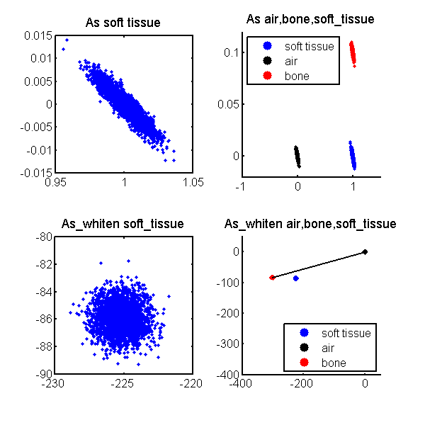
Figure 1 Scatterplots of original and whitened A-vector data. The top two panels show the scatterplots of the data in the soft tissue only region of the phantom (see the previous post). The top two panels show the original A-vector data and the bottom panels show the whitened data.

Optimal SNR conventional image

Combining the ideas of the previous two sections, we can maximize the SNR of a conventional image computed from A-vector data by forming a dot product of the whitened data with a unit vector in the direction of the vector from the background to the object in the whitened coordinates. The vector from the air to the bone data is drawn in the lower right panel of Fig. 1↑. Notice that the angle of the vector to the soft tissue data is not much different than for the bone data so the soft tissue SNR will also be close to optimal.

The images

Conventional total photon number and optimal projection images computed as discussed in this post are shown in Fig. 12 of the paper..

Conclusion

The image shows that the optimal projection images from A-vector data have a somewhat better SNR than the conventional total photon number images.

--Robert Alvarez

Last edited Sep 11, 2014

Linking is allowed but reposting or mirroring is expressly forbidden.