If you have trouble viewing this, try the pdf of this post. You can download the code used to produce the figures in this post.
Estimator parameters
You may ask, what is the fundamental advantage of the new estimator? Yes, it is faster than the iterative method but so what? With Moore’s law, we can just throw silicon at the problem by doing the processing in parallel. I have two responses. The first is that not only is the iterative estimator slow but it also takes a random time to complete the calculation. This is a substantial problem since CT scanners are real-time systems. The calculations have to be done in a fixed time or the data are lost. The gantry cannot be stopped to wait for a long iteration to complete!
The second problem is that, as it has been implemented in the research literature, the iterative estimator requires measurement of the x-ray tube spectrum and the detector energy response to compute the likelihood for a given measurement. These are difficult measurements that cannot be done at most medical institutions. Because of drift of the system components, the measurements have to be done periodically to assure accurate results. There may be a way to implement an iterative estimator with simpler measurements but I am not aware of it.
In this post, I will show how the parameters required for the new estimator can be determined from measurements on a phantom placed in the system. This could be done easily by personnel at medical institutions and is similar to quality assurance measurements now done routinely on other medical systems.
The calibrator
The calibrator is a physical device provided by the manufacturer that would be placed in the x-ray system by medical institution personnel. They would then invoke a program, again provided by the manufacturer, to acquire x-ray data on the transmission through the phantom with the source spectra and detector responses used in energy selective patient scans. The program would use these data to compute an update to the estimator parameters to account for drift in the x-ray source and detector responses.
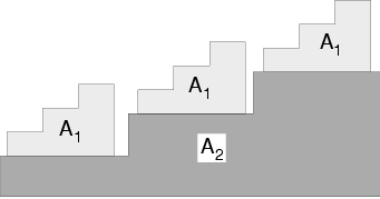
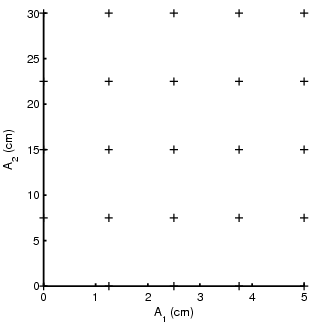
The calibrator is shown in Part (a) of Fig. 1↓. It consists of a set of accurately machined step wedges composed of two materials such as plastic and aluminum. The thicknesses of steps are pre-determined to give a rectangular points when plotted in two dimensions as shown in Part (b) of the figure. The thicknesses could be adjusted to compensate for different slant lengths for detectors that are off center in a fan beam system.
The linear MLE
I will first discuss how the parameters of the linear maximum likelihood estimator are computed from the calibrator data. The linear MLE is derived in Sec. II.A of the paper
The estimator is implemented as a matrix multiplication where the term in brackets in Eq. 1↑ is a constant matrix that only depends on the system parameters. During a scan, the measured data L for each line through the object are multiplied by the matrix to give the estimate. The L vector is actually the negative of the logarithm of the measurements for each spectra divided by the corresponding measurements with no object in the system. These could be determined during the calibration process before the phantom is placed in the system.
To compute the constant matrix, we need to determine the M and R matrices from the calibrator data. As discussed in the paper, the M matrix is the gradient of the measurement vector as a function of A-vector
(2) M = (∂L)/(∂A).
Theoretically, the gradient is evaluated at the operating point but, for the purpose of the estimator, I used the average value over all the calibration data. The M matrix is then the coefficients of the least squares fit of the calibration data Lcalib as a function of the calibrator A-vectors. In Matlab notation,
(3) M = Acalib\Lcalib.
This can be understood as follows. Suppose L and A are linearly related so
L1
=
m11A1 + m12A2
L2
=
m21A1 + m22A2
.
Then, for example,
(∂L1)/(∂A1) = m11
and so on for all the elements of the M matrix.
The R matrix is the covariance of the measurement data. Again, theoretically it is the covariance for the operating point but the estimator uses a value for the center of the calibration region. The calibration phantom steps are actually rectangles so the data for each step provide samples of the data with constant A-vector. We can then compute the R matrix as the sample covariance of the data for a single step.
The correction table
Once we have the linear MLE, we can use it with the calibrator data to compute the correction table. The corrections are the difference between the linear MLE estimate and the actual thicknesses of the calibrator step wedge for each step. An example is shown in Fig. 2↓. Code to reproduce the figures is available here.
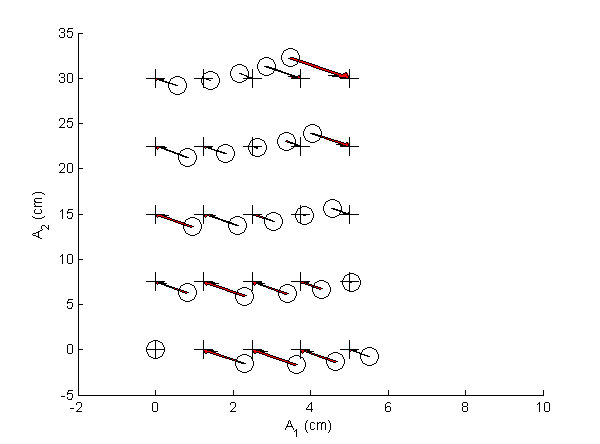
Correction table look up
During the operation of the estimator, the input to the correction table is the linear MLE estimate. As shown in Fig. 2↑, these are not on a rectangular lattice so we cannot apply standard functions such as Matlab’s interp2. In the implementation for the paper, I used John D’Errico’s gridfit function. In the function documentation, he says
Gridfit is not an interpolant. Its goal is a smooth surface that approximates your data, but allows you to control the amount of smoothing.
You can see the gridfit parameters I used in the code for the AtableSolveEquations function.
Another problem is that noise may produce linear MLE estimates that are outside the region spanned by the calibration data. Unlike most interpolating (or function approximating to be more precise functions, gridfit will extrapolate. However, although AtableSolveEquations has code to implement this, I did not use that feature. Instead I chose the nearest point on a line from the point with noise to the centroid of the calibration data. The method is described in detail in Section II.D and Fig. 5 of the paper. See also the code in AtableSolveEquations.
Conclusion
The ability to derive the estimator parameters from measurements with the x-ray system hardware without requiring specialized instruments is a major advantage for the new estimator. It makes possible the use of the estimator routinely in clinical settings instead of just as a demonstration of the feasibility of the technique.
--Bob Alvarez
Last edited Dec 26, 2013
Copyright © 2013 by Robert E. Alvarez
Linking is allowed but reposting or mirroring is expressly forbidden.