If you have trouble viewing this, try the pdf of this post. You can download the code used to produce the figures in this post.
Rationale for the new estimator
The past two posts have discussed estimators for A-vector data. I showed that with the same number of measurement spectra as the A-vector dimension, any estimator that solves the deterministic equations is the maximum likelihood estimator (MLE) and it will achieve the Cramèr-Rao lower bound (CRLB). If there are more measurement spectra than the dimension, then the polynomial estimator, which works well for the equal case, has very poor performance giving a variance that can be several hundred times larger than the CRLB. I showed by simulations that with more measurements than dimension the iterative MLE does give a variance close to the CRLB but it has substantial problems. Common to all iterative algorithms, the computation time is long and random. It may fail to converge at all if the initial estimate is too far from the actual value. As it was implemented by Schlomka et al.[2], it also requires measurements of the x-ray source spectrum and the detector spectral response. These are difficult, time consuming and require laboratory equipment that is not usually available in medical institutions.
In this post, I will give an intuitive explanation for the operation of a new estimator that I introduced in my paper[1] “Estimator for photon counting energy selective x-ray imaging with multi-bin pulse height analysis,” which is available for free download here. The estimator is efficient and can be implemented with data that can be measured at medical institutions. The details of the estimator are described in the paper. Here, I will discuss the background and give a rationale on how it works.
The linear MLE with constant covariance
The estimator uses a two step algorithm. First it computes the linear MLE of the measured data. Then it applies a correction to the linear estimate since the transformation L(A) is not quite linear. The first question you might ask is why should this give a noise variance close to the CRLB? The answer to this question depends on the properties of the linear MLE, which I will discuss in this section.
I discussed the linear MLE in a previous post. It makes two important assumptions: (1) the measurements L and the A-vector are linearly related and (2) the covariance is constant. I will examine the linear assumption first. With this assumption, the measurements are given by
(1) Lwith_noise = MA + w.
In this equation, Lwith_noise is the negative of the log of the measurements divided by the measurements with no object in the system. The M matrix is the effective attenuation coefficients, A is the vector of the line integrals of the basis set coefficients, and w is zero mean multivariate normal noise.
The plot of L versus A in Fig. 1↓ shows that the linear approximation is actually quite good so the errors will probably be small. Furthermore, the errors correspond to a small offset or bias of the mean value but, as shown next, the random variations for each point are close to the values that would be produced by a MLE using an accurate model.
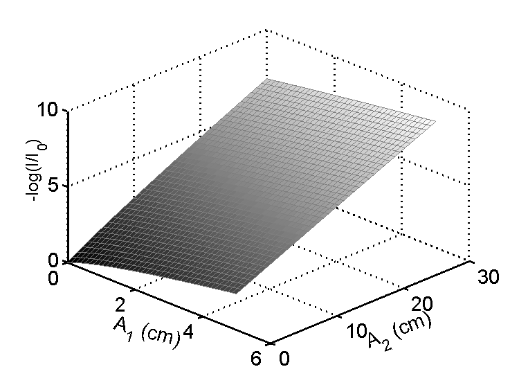
Figure 1 L vs. A for an 80 kilovolt x-ray tube spectrum and an aluminum/plastic basis set. Notice that the transformation is nearly linear. This is a plot of one of the components of L. The other components give similar results. This plot is from my previous post “Applying statistical signal processing to x-ray imaging.” You can download the code package for that post to reproduce the graph.
The noise performance depends on the second assumption of the linear MLE that the covariance is constant. This seems to be more problematic. After all, the covariance of the log measurements, CL, is proportional to 1⁄Nphotons and the number of photons varies as a (negative) exponential of the thickness so it is definitely not a constant. However, if we study the formula for the linear MLE from my previous post,
we notice an interesting property. The estimator, which is the matrix in brackets in Eq. 2↑, does not change if we multiply the covariance by a constant. Since (kCL) − 1 = 1⁄kC − 1L, where k is a scalar constant, the first factor in the bracket in Eq. 2↑, (MTC − 1LM) − 1, is proportional to k and the second factor, MTC − 1L, is proportional to 1⁄k so the two factors cancel out and the matrix is unchanged if CL is replaced by kCL.
Because low x-ray energy measurements are attenuated more than high energy measurements, the effect of thickness increase is not simply to multiply by a constant. Instead, relative sizes of the elements of CL change as the thickness varies . However the change is relatively small and does not cause the variance to become substantially larger than the CRLB. The reason for this is related to the linear constant covariance CRLB being a good approximation to the full CRLB that I noted in a previous post. Fig. 1 of that post (reproduced as Fig. 2↓ of this post), shows that the constant covariance CRLB is essentially equal to the full CRLB for small object thicknesses where the photon counts are above a few hundred.
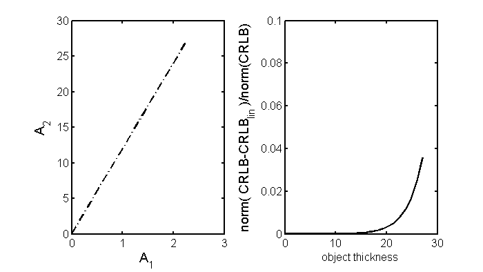
Figure 2 Fractional error of constant covariance CRLB compared with the full CRLB. The left panel shows the path through A-space and the right panel shows the error as a function of the distance from the origin along that line. This distance is proportional to the thickness of an object with an a-vector with ratio of components equal to the slope of the line in the left panel. The graph is from this post and you can download the code package from that post to reproduce the figure.
Similarly, as shown in Fig. 3↓, which is Fig. 12 of my paper, the main deviation of the variance of the linear MLE from the CRLB occurs for thick objects. However, as shown in the figure, the deviation is quite small and much smaller than the deviation of the polynomial estimator variance.
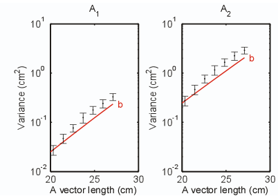
Figure 3 Variance of new estimator errors for large object thickness. The error bars are the standard deviation of the estimates of the variance with the Monte Carlo simulation of the estimator. Note that the variance becomes slightly larger than the CRLB, which is the solid red line, as the thickness increases. As discussed in this post, this is similar to the errors in the constant covariance approximation to the the CRLB increasing as the thickness increases and the number of photons decreases.
Conclusion
The arguments presented here show why starting with the linear MLE is a good idea. Unlike the polynomial estimator, the linear MLE properly weights the measurements so the lower noise data have the strongest influence on the estimate. The MLE uses the probability distribution function of the measurements to handle the cases where the noisy data are not on the calibration surface. As shown in my paper[1], the errors in the linear MLE can be corrected after the fact to give the optimal noise variance of the MLE with negligible bias. In my next post, I will describe how we can implement the new estimator using data measured by the x-ray system itself without requiring additional specialized physics instruments or putting the medical scanner off line for substantial times.
Last edited Nov 01, 2013
Copyright © 2013 by Robert E. Alvarez
Linking is allowed but reposting or mirroring is expressly forbidden.
References
[1] : “Estimator for photon counting energy selective x-ray imaging with multi-bin pulse height analysis”, Med. Phys., pp. 2324—2334, 2011.
[2] : “Experimental feasibility of multi-energy photon-counting K-edge imaging in pre-clinical computed tomography”, Phys. Med. Biol., pp. 4031—4047, 2008.