Estimators for Energy-selective imaging—Part 1
In a
previous post I described the application of statistical estimator theory to energy selective x-ray imaging. I introduced a linearized model for the signal and noise and in a subsequent
post I described a linear maximum likelihood estimator (MLE) that achieved the Cramèr-Rao lower bound (CRLB). In many applications, such as CT, the linear model is not sufficiently accurate. In this post, I will start the discussion of my paper
[3] “Estimator for photon counting energy selective x-ray imaging with multi-bin pulse height analysis.” The paper describes an estimator that is accurate for a wide dynamic range that also achieves the CRLB and has other desirable properties such as fast and predictable computation time and being implementable in a clinical institution as opposed to a physics lab. This post frames the discussion by describing general aspects of computing the A-vector from energy selective measurements and several estimators that are widely used and their properties.
edit: I added a plot of the ratio of the least squares estimator variance to the CRLB variance for least squares estimator when the number of bins is larger than the A-vector dimension. Added detail to the MLE when the number of measurements and dimension are equal.
edit 2: I changed the name of the “least squares estimator” to “multinomial approximation estimator.”
Estimation as a transformation
In my
previous post, I derived the fundamental equations relating the A-vector to the x-ray measurements
In these equations,
λk(A) is the total counts in measurement
k. It will soon become clearer why I use
λ for the counts. The source photon number spectrum is
nsource(E) and
Aj is the line integral of the coefficient of the
j − th basis function
fj(E). The energy response of each measurements is
dk(E), which can be the energy response of bin
k with PHA or the k-th switched source spectrum,
dk(E)nsource(E) . Although the theory is applicable to integrated energy measurements, as shown in
my dissertation, I will assume here that we use photon counting detectors.
If we have two measurements, as has been the case throughout most of the history of energy selective imaging, hence the name dual energy imaging, then we can consider Eqs.
1↑ to define a transformation between the two-dimensional spaces, the A-vector and the measurement vector. In
my paper, I discuss this at some length and show that under reasonable conditions, such as the effective spectra being different and the basis functions linearly independent, the transformation is invertible.
The multinomial approximation estimator
Although we know that the transformation is invertible, how do we invert it? The most common approach is to approximate the components of the A-vector with a second order multinomial in the log of the individual measurements.
I call this the multinomial approximation estimator because the coefficients
cjk are calculated from a least squares multinomial fit to a set of calibration data such as with a step wedge phantom made from two materials and with many combinations of thicknesses. In this case, we can use the attenuation coefficients of the calibration materials as the basis set so the A-vector components are simply the thicknesses of the two materials
[2].
This method has been widely used but has several problems. One is that, with PHA, we can have many more measurements than the dimension of the A-vector. It is easy enough to generalize Eqs.
2↑ but what does this do to the noise? We need to apply statistical estimator theory to answer this question.
MLE when the number of measurements and dimension are equal
Statistical estimator theory
[4] provides many approaches to designing estimators. The maximum likelihood estimator (MLE) is widely used because it is (relatively) easy to implement and has good statistical properties. For example, it is known to achieve the CRLB for a large number of observations. In my 1976 paper
[1], I discussed the MLE when the number of measurements and dimension are equal. With negligible pileup, the counts can be modeled as independent Poisson random variables. The distribution of the counts in each energy bin is
where
λk(A) is the expected value of the counts in bin
k, given by Eq.
1↑. As indicated, it is a function of the A-vector,
A. Since the bin counts are independent, their joint distribution is the product of the individual marginal distributions and the log of the joint distribution is the sum of the logs of the distributions of the bins
where K is the number of spectra or PHA bins.
To find the MLE, we consider Eq.
4↑ to define a function of
A for a fixed set of measurements
nk, differentiate with respect to
A and set the derivative equal to zero. Carrying out the operation
Evaluating this equation for all the components of
A results in two homogeneous linear equations for the quantities
nk⁄λk − 1.
(∂ℒ)/(∂A1)⎛⎝(n1)/(λ1) − 1⎞⎠
+
(∂ℒ)/(∂A1)⎛⎝(n2)/(λ2) − 1⎞⎠
=
0
(∂ℒ)/(∂A2)⎛⎝(n1)/(λ1) − 1⎞⎠
+
(∂ℒ)/(∂A2)⎛⎝(n2)/(λ2) − 1⎞⎠
=
0
With the number of measurements and dimension equal, the unique solution is
That is
n1 = λ1 and
n2 = λ2. This is valid if the determinant of the coefficients is not equal to zero. For the two dimension case with two measurements this is
This equation says that the Jacobian of the transformation from
λ to
A is not zero. If this is true, then Eqs.
6↑ and therefore the MLE are solved by setting the expected value of the measurements equal to the measured photon counts. That is, solve the deterministic equations with the measured data. One way to do this is with the multinomial approximation estimator in Eq.
2↑and in this case it is also the MLE.
multinomial approximation estimator with more measurements than dimensions
If the number of measurements is greater than the dimension, then there is no unique solution to Eqs.
5↑. We can generalize the multinomial approximation estimator in Eq.
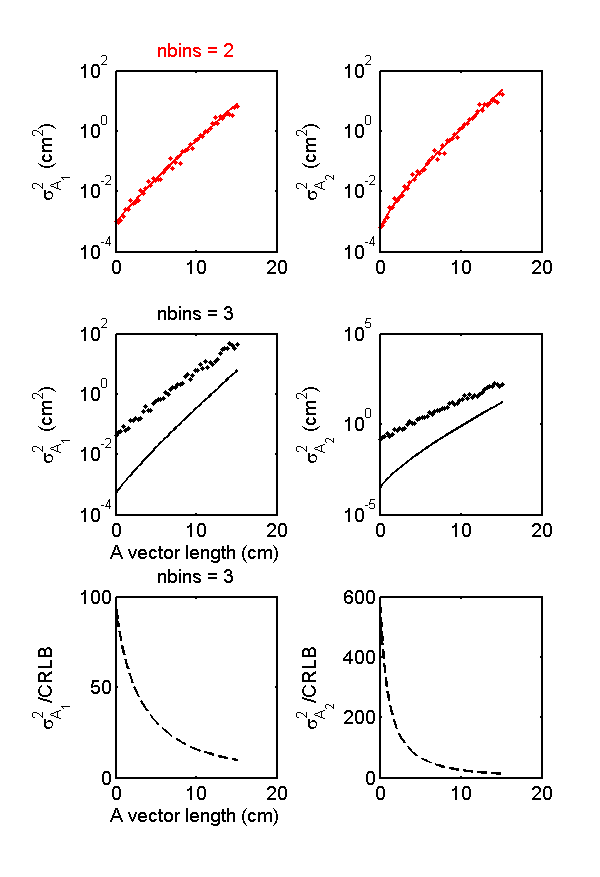
2↑ for more measurements as we have sufficient calibration data to determine the coefficients with a least squares algorithm. However, now there is no guarantee that the multinomial approximation result is the MLE or that it achieves the CRLB. Fig.
4↓ shows that if the number of spectra is greater than the A-vector dimensions, the multinomial approximation estimator does not achieve the CRLB. Instead the variance is several hundred times larger than the CRLB, an obviously undesirable result!
MLE with more measurements than dimensions—the iterative implementation
Another approach to solving the equations when the number of measurements is greater than the dimension is to maximize Eq.
4↑ iteratively. This is the algorithm described by Roessl and Proksa
[5] that was used in an experimental system by Schlomka et al.
[6]. Their approach assumed that you know the source energy spectrum and the energy response of individual PHA bins. Their experimental implementation was a technical tour-de-force where they measured the spectrum with high resolution multi-channel analyzers and the detector energy response at a synchrotron radiation laboratory.
For their implementation, we can start with the Eq.
4↑ for the likelihood. We can search for the maximum iteratively if we have a way to compute
λk(A). If we know the source spectrum
nsource(E) and the detector energy response
dk(E), and we have tabulated data for the attenuation coefficients of the basis materials
fk(E), then we can use Eq.
1↑ to compute
ℒ and use an iterative algorithm like Matlab’s fminsearch to maximize the log-likelihood. The implementation actually minimizes the negative, which is equivalent to maximizing.
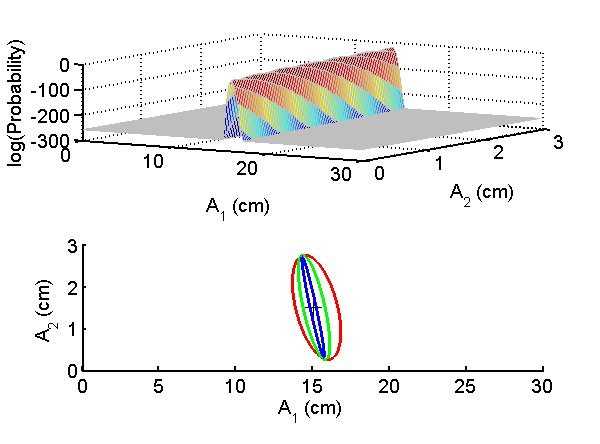
A possible problem is that multiple local maxima keep us from finding the overall maximum. Figs.
2↑ and
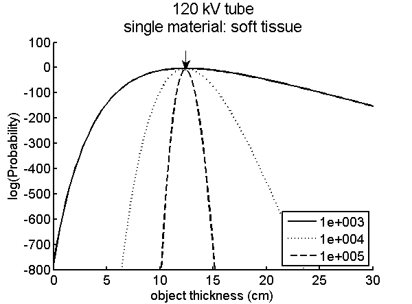
3↑ show the the log-likelihood functions are well behaved. Fig.
2↑ is a plot of the log-likelihood function for the one dimension case. The function is plotted for several values of the photon counts and you can see that it has only one peak that becomes sharper and therefore the variance of the random errors decreases as the number of photons increases. Fig.
3↑ shows that this is also the case with a two dimension basis set. Notice that the contours in the bottom panel are not circular so the errors in the two components will not have the same variance and they will be negatively correlated.
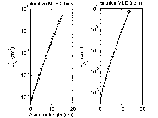
Fig.
4↑ shows the Monte Carlo variance and the CRLB for the iterative MLE three bin case. Comparing this with the bottom row of Fig.
1↑, the variance is much smaller with the iterative than with the multinomial approximation estimator
Conclusion
The multinomial approximation estimator has good performance if the number of measurements is equal to the A-vector dimension but has poor performance with more measurements. The iterative MLE has good performance even if the number of measurements is greater than the dimension but it has many problems. One is that the implementation I describe requires measurements of the source spectrum and the detector energy response. These are difficult measurements that require instruments not commonly available in clinical institutions. The measurements have to be repeated periodically since the system components drift with age. The iterative algorithm also has computation problems. It is complicated and can fail to converge. Perhaps more importantly it does not have a fixed computation time, which is required for real time performance with medical equipment. In the next post, I will describe an algorithm that addresses these problems.
Acknowledgment
The code for this post includes a Poisson random number generator by Jeff Fessler that I translated from Octave to Matlab for those who do not have the Matlab statistical toolbox with its poissrnd function.
Last edited Feb 04, 2016
Copyright © 2013 by Robert E. Alvarez
Linking is allowed but reposting or mirroring is expressly forbidden.
References
[1] R. E Alvarez, A. Macovski: “Energy-selective reconstructions in X-ray computerized tomography”, Phys. Med. Biol., pp. 733—44, 1976.
[2] Robert E Alvarez, Edward J Seppi: “A comparison of noise and dose in conventional and energy selective computed tomography”, IEEE Trans. Nucl. Sci., pp. 2853—2856, 1979.
[3] Robert E. Alvarez: “Estimator for photon counting energy selective x-ray imaging with multi-bin pulse height analysis”, Med. Phys., pp. 2324—2334, 2011. URL http://www.ncbi.nlm.nih.gov/pubmed/21776766.
[4] Steven M. Kay: Fundamentals of Statistical Signal Processing, Volume I: Estimation Theory . Prentice Hall PTR, 1993.
[5] E. Roessl, R. Proksa: “K-edge imaging in x-ray computed tomography using multi-bin photon counting detectors”, Phys. Med. Biol., pp. 4679—4696, 2007.
[6] J P Schlomka, E Roessl, R Dorscheid, S Dill, G Martens, T Istel, C Bäumer, C Herrmann, R Steadman, G Zeitler, A Livne, R Proksa: “Experimental feasibility of multi-energy photon-counting K-edge imaging in pre-clinical computed tomography”, Phys. Med. Biol., pp. 4031—4047, 2008.