aprendtech.com >> blog >> this post

If you have trouble viewing this, try the pdf of this post. You can download the code used to produce the figures in this post.

NQ detector stats

Another way to get energy selective data is to measure the total number of counts and their total energy. This may not seem to provide energy-dependent information but if you look at it from the point of view of energy weighting, there is information. We can look at the total counts as the integral of the spectrum multiplied by a constant function of energy, where the constant is one. On the other hand, the total energy is the integral of the spectrum multiplied by the function f(E) = E. This weights the higher energies more than the lower and therefore has different information than the counts. This is actually enough difference to give SNR comparable to two-bin PHA.

I call this NQ since I use the symbols N for counts and Q for total energy but its inventors called it the CIX detector for simultaneously Counting and Integrating X-ray detector. The concept was originally introduced by Overdick et al.[2] to address the count rate problem with the idea to use the count signal at low count rates and the integrated energy at high count rates. Later Roessl et al.[3] noticed that the two quantities provide energy selective information and showed that the positive correlation between N and Q helps to reduce the variance of the output A-vector signal.

In this post, I will derive the expected value and covariance of the N and Q signals. We can then use these results with the statistical detection theory method of my paper[1] to compute the SNR and to compare it to other types of detectors and to the optimal SNR.

Expected value and variance of photon counts and total energy

The counts have a Poisson distribution so the expected value and variance are equal to the Poisson parameter λ.

⎡⎢⎣ ⟨N⟩ = λ σ²_N = λ ⎤⎥⎦

The total energy is a compound Poisson random variable since it is the sum of a random number of random photon energies.

Q = ^N⎲⎳_k = 1E_k

The probability distribution function of the energies is the spectrum normalized so its integral is equal to one

p_E(E) = (S(E))/(⌠⌡S(E)dE)

We can derive the expected value and variance of Q using its moment generating function (MGF), which can be derived from its definition M_Q = ⟨e^tQ⟩ as shown in Eq. 1↓

(1) M_Q(t) = ⟨e^tQ⟩ definition = ⟨⟨e^{tⁿ⎲⎳_k = 1E_k}⟩|N = n⟩ conditional expectation = ⟨⟨e^tE₁⋯e^tE_n⟩|N = n⟩ = ⟨⟨e^tE⟩ⁿ|N = n⟩ E_k i.i.d. = ⟨M_E(t)ⁿ|N = n⟩ M_E(t) = ⟨e^tE⟩ by definition = ⟨e^n(log M_E)|N = n⟩ = M_N(log M_E)

M_Q in Eq. 1↑ is valid for all probability distributions of the count variable N. If N is Poisson, its MGF is

M_N(t_N) = exp[λ(e^t_N − 1)]

Substituting in (1↑), the MGF becomes

(2) M_Q(t) = exp[λ(M_E(t) − 1)]

The expected value can be calculated from the first derivative of (2↑) evaluated at t = 0

(3) ⟨Q⟩ = ⎡⎣(∂M_Q)/(∂t)⎤⎦_t = 0 = λexp[λ(M_E(t) − 1)](∂M_E)/(∂t)|_t = 0

From the definition, it is a general property of any MGF that

M(0) = 1 (∂M_E)/(∂t)(0) = ⟨E⟩

Using these in (3↑)

⟨Q⟩ = λ⟨E⟩

Variance of Q

Differentiating the first derivative (3↑) again

(4) (∂²M_Q)/(∂t²) = λexp[λ(M_E(t) − 1)]⎡⎣(∂²M_E)/(∂t²) + λ⎛⎝(∂M_E)/(∂t)⎞⎠²⎤⎦.

Evaluating (4↑) at t = 0, and noting that ⎡⎣(∂²M)/(∂t²)⎤⎦_t = 0 = ⟨E²⟩

⟨Q²⟩ = λ⟨E²⟩ + λ²⟨E⟩².

The variance of Q can then be computed from the general formula for the variance

var(Q) = ⟨Q²⟩ − ⟨Q⟩² = λ⟨E²⟩ + λ²⟨E⟩² − λ²⟨E⟩² = λ⟨E²⟩

Covariance of N and Q

We can compute the covariance using the general formula

(5) cov(N, Q) = ⟨NQ⟩ − ⟨N⟩⟨Q⟩.

The expected value of the product can be computed using conditional expectation

⟨NQ⟩ = ⟨n⟨^N⎲⎳_k = 1E_k⟩|N = n⟩ conditional expectation = ⟨n²⟨E⟩|N = n⟩ E_k iid = ⟨E⟩(λ + λ²)

The last step follows because the second moment of the Poisson is ⟨N²⟩ = σ²_N + ⟨N⟩² = λ + λ²

Substituting in (5↑), the covariance is

cov(N, Q) = λ⟨E⟩ + λ²⟨E⟩ − λ²⟨E⟩ = λ⟨E⟩.

The covariance matrix is therefore

(6) cov(N, Q) = λ⎡⎢⎣ 1 ⟨E⟩ ⟨E⟩ ⟨E²⟩ ⎤⎥⎦

Expected value and variance of logarithm signals

We can use these formulas with the general results for the logarithm of signals from my previous post to derive the parameters. In the previous post I derived the expected value and variance of the log of counts.

⟨log(N)⟩ = log(λ) var(log(N)) = (1)/(λ)

The validity of the log formulas in that previous post was justified for photon counts but since both the expected value and variance of Q are proportional to λ, the previous justifications are also applicable to Q. The log parameters are then

(7) ⟨log(Q)⟩ = log(⟨Q⟩) var(log(Q)) = (var(Q))/(⟨Q⟩²) = (F)/(λ) cov(log(N), log(Q)) = (cov(N, Q))/(⟨N⟩⟨Q⟩) = (1)/(λ)

where the excess variance factor F = ^⟨E²⟩⁄_⟨E⟩².

The covariance matrix of the log data is

(8) cov(log(N), log(Q)) = (1)/(λ)⎡⎢⎣ 1 1 1 F ⎤⎥⎦

Monte Carlo simulation

I tested these formulas with a Monte Carlo simulation. As usual, you can download the code to reproduce these features. Since the distribution of the counts is Poisson, which is well-known, I did not plot the results although you can examine them when you run the code. Fig. 1↓ plots the statistics of the total energy Q.

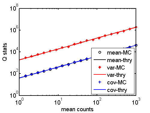
Figure 1 Monte Carlo test of Q statistics. Shown are the expected value, the variance, and the N,Q covariance. As you can see from Eq. 6↑, the NQ covariance is equal to the Q expected value so the data overlap.

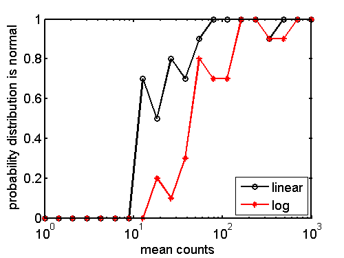
I discussed statistical tests for normally distributed data in a previous post. Basically they are extensions of the normal probability plot, which plots the sorted data using distorted coordinates so normally distributed data will fall on a straight line. Deviations from the line may indicate that the data are not normally distributed. The results of the test are themselves random so the code implements repeated tests for each counts value that are then averaged using a value of “1” for the normal hypothesis and “0” to reject the hypothesis. The averaged results to give a “probability” to accept the normal distributed hypothesis. We would expect and Fig. 2↓ shows that the probability increases as the mean counts increase.

Figure 2 Probability to accept multivariate normal distribution for N,Q data versus the expected counts. The probability was tested using Royston’s algorithm[4] as implemented by the Matlab function roystest.m[5].

Conclusion

I have derived formulas for the parameters of a multivariate normal distribution, the expected values and covariance, for the NQ detector. I verified the formulas with a Monte Carlo simulation. I also showed that the multivariate normal is a valid probability distribution model for counts greater than about 100 for linear data and 500 for log data. I will use the formulas in later posts to compute the SNR using the approach of my paper[1]

—Bob Alvarez

Last edited Aug 02, 2012

Linking is allowed but reposting or mirroring is expressly forbidden.

References

[1] Robert E. Alvarez: “Near optimal energy selective x-ray imaging system performance with simple detectors”, Med. Phys., pp. 822—841, 2010.

[2] Michael Overdick, Walter Ruetten, Thomas Zaengel: US Patent No. 6759658 - X-ray detector having a large dynamic range. 2004.

[3] Ewald Roessl, Andy Ziegler, Roland Proksa: “On the influence of noise correlations in measurement data on basis image noise in dual-energy like x-ray imaging”, Med. Phys., pp. 959—966, 2007.

[4] J. P. Royston: “Some Techniques for Assessing Multivarate Normality Based on the Shapiro- Wilk W”, Journal of the Royal Statistical Society. Series C (Applied Statistics), pp. 121—133, 1983.

[5] A. Trujillo-Ortiz, R. Hernandez-Walls, K. Barba-Rojo, L. Cupul-Magana: Roystest: Royston's Multivariate Normality Test. A MATLAB file.. URL MATLAB Central File Exchange, http://www.mathworks.com/matlabcentral/fileexchange/17811.