If you have trouble viewing this, try the pdf of this post. You can download the code used to produce the figures in this post. Edited May 12, 2012 to clarify that constant covariance log data and photon count data give same formula for the CRLB.
SNR with PHA vs. number of bins
In this post, I will discuss the signal to noise ratio (SNR) of a photon counting detector with pulse height analysis (PHA). I will show that it approaches the ideal full-spectrum SNR as the number of bins gets large. I will also show that we can get quite close to the ideal value even with a small number of bins, which was one of the main points in my paper.
I will begin by re-visiting a result from my last post that the Cramèr-Rao lower bound (CRLB) with multivariate normal log of photon count data assuming a constant covariance is nearly equal to the accurate matrix that includes the variation of the covariance. The derivation becomes problematic with a large number of bins since the mean value in each bin may be small enough so the normal approximation to the counts is not valid. I will show an alternate derivation that uses the Poisson model of the count data, which is valid for small counts. The result is formally the same as with the normal approximation so the CRLB formula can be applied for any number of bins. This result is new and was not included in my paper.
Imaging task for SNR with A-space data
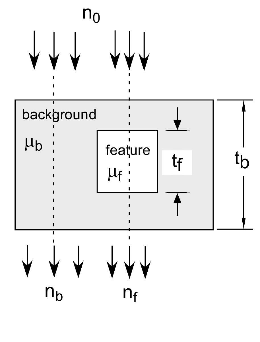
Summarizing my previous development, to determine the SNR with energy spectrum information I analyzed the imaging task shown in Fig. 1↓. I introduced the A-space description by using the attenuation coefficients of the background μb and feature μf materials as the basis function. With this basis set, the a vectors for the feature and background materials are simply
af = ⎡⎢⎣
1
0
⎤⎥⎦, ab = ⎡⎢⎣
0
1
⎤⎥⎦.
The A-vector in the background region is Ab = tbab while in the feature region it is Af = (tb − tf)ab + tfaf . We can apply the statistical detection theory model described in my previous post by assuming that the A-vector data are described by a multinormal distribution with expected values under two hypotheses: ⟨AH0⟩ = Ab and ⟨AH1⟩ = Af and a covariance CA. From my last post, the performance will depend only on the signal to noise ratio
(1) SNR2 = δATC − 1AδA
where δA = ⟨AH1⟩ − ⟨AH0⟩ = tf(af − ab).
δA
=
⟨AH1⟩ − ⟨AH0⟩
=
tf(af − ab)
=
tf⎡⎢⎣
1
− 1
⎤⎥⎦
In general, the covariance of the A-space data depends on the estimator used. But we know that the ’minimum’ covariance (suitably defined for matrix data) is the CRLB, so we can determine the optimal performance by using it for the covariance CA. In a previous post, I showed that we could use a linearized model with multivariate normal noise data. With this model, the CRLB is
where M = (∂L)/(∂A) is the gradient of log of the x-ray measurements in A-space evaluated at the operating point of the model and CL is the covariance of the log data with noise. The SNR with the imaging task in Fig. 1↓ is
CRLB with complete energy information
I would like to apply this model to show that the SNR approaches the full spectrum as the number of bins becomes large. However, as mentioned, with a large number of bins the data may not satisfy the assumptions of a large number of counts. In that case, I will use a Poisson model, which is valid for small mean counts, to show that the same formula (2↑) can be used in all cases.
I will derive the CRLB for independent multivariate Poisson data. As I have discussed in a previous post, this is a good model for the PHA counts if the deadtime is negligible compared to the mean inter-arrival time of the photons. Table 1↓ lists the notation I use in this post.
It is convenient to use the Fisher information matrix F, which is the inverse of the CRLB. As shown in Theorem 3.2 of Kay[1], F has components which are the negative of the expected value of the second derivative of the log of the likelihood ℒ = log[Pr(N;A)]
Fij = − ⟨(∂2ℒ)/(∂Ai∂Aj)⟩
The bin counts nk are independent Poisson random variables, which have a distribution function
Pr(nk;A) = (e − ⟨nk⟩⟨nk⟩nk)/(nk!) = (e − gk(A)gk(A)nk)/(nk!)
where the expected value ⟨nk⟩ = gk(A) is assumed to be a function of the A-vector. Since the nk are independent the joint probability is the product of the distributions and the log of the likelihood is
ℒ = K⎲⎳k = 1[ − gk + nklog(gk) − log(nk!)].
To evaluate the Fisher information, we need the derivatives. The first derivative can be expressed as a matrix product of the gradient of g, the inverse of the photon count covariance C − 1, and the difference of the measured data and the expected values. Since the count data are independent, their covariance matrix and its inverse are
C = ⎡⎢⎢⎢⎣
g1
0
⋯
0
gK
⎤⎥⎥⎥⎦, C − 1 = ⎡⎢⎢⎢⎣
1⁄g1
0
⋯
0
1⁄gK
⎤⎥⎥⎥⎦
(∂ℒ)/(∂Aj)
=
⎲⎳⎡⎣(∂gk)/(∂Aj)⎛⎝(nk − gk)/(gk)⎞⎠⎤⎦
=
(∂gT)/(∂Aj)⎡⎢⎢⎢⎣
1⁄g1
0
⋯
0
1⁄gK
⎤⎥⎥⎥⎦(N − g)
=
(∂gT)/(∂Aj)C − 1(N − g)
Note that this covariance is valid even with small number of counts per bin.
The second derivative is
(∂2ℒ)/(∂Ai∂Aj) = (∂)/(∂Ai)⎡⎣(∂gT)/(∂Aj)C − 1⎤⎦(N − g) − (∂gT)/(∂Aj)C − 1(∂g)/(∂Ai).
The expected value of the first term is zero since the term in the bracket does not depend on the data and⟨N⟩ = g. The second term does not depend on the data so
Fij
=
− ⟨(∂2ℒ)/(∂Ai∂Aj)⟩
=
(∂gT)/(∂Aj)C − 1(∂g)/(∂Ai)
The full matrix is
where I have used the notation of van den Bos[2] Appendix D so
(∂g)/(∂AT) = ⎡⎢⎢⎢⎣
(∂g1)/(∂A1)
(∂g1)/(∂A2)
⋯
(∂g2)/(∂A1)
(∂g2)/(∂A2)
⋯
⋯
⋯
⋯
⎤⎥⎥⎥⎦
and ⎛⎝(∂g)/(∂AT)⎞⎠T = (∂gT)/(∂A).
If the number of bins is large so the energy width is small, we can use the Beer’s law exponential model of the expected value of the counts
gk(A) = ⟨nk⟩ = nk0exp[ − μk1A1 − μk2A2]
where nk0 is the mean of the number of photons incident on the object in the k’th energy bin. Differentiating,
(∂gk)/(∂Ai) = − μkigk.
We can express all the components as a matrix multiplication
(∂g)/(∂AT) = − MTC
where I have used the fact that all covariance matrices are symmetrical so CT = C.
The Fisher information matrix derived in my previous post assuming log data is F = MTC − 1LM (see Eq. 8 of my previous post, which I reproduce here)
(6)
cov(ÂMLE)
=
(MTC − 1LM) − 1
Recall that the CRLB is the inverse of F, so the Fisher information matrix from my previous post is the term in the parentheses of Eq. 6↑. With photon count data, the variance is the inverse of the number of counts and since CL is a diagonal matrix, C − 1L = C. Thus Eq. 5↑ has the same form as the Fisher information of constant covariance multivariate normal data, derived in my previous post but here it is derived without the assumptions that the covariance is constant and the mean count values are large. Therefore, we can use the same formula (2↑) for the covariance of the A-space data for any number of bins.
SNR for K bin PHA
To derive the SNR with K-bin data, we need to evaluate Eq. 3↑ with
δA = tf⎡⎢⎣
1
− 1
⎤⎥⎦, M = ⎡⎢⎢⎢⎣
M11
M12
⋯
⋯
MK1
MK2
⎤⎥⎥⎥⎦, C = ⎡⎢⎢⎢⎣
⟨n1⟩
0
⋯
0
⟨nK⟩
⎤⎥⎥⎥⎦.
This is straight-forward but tedious, so I used Maxima to automate the matrix computation. Maxima is an open-source symbolic math program that is available for download here. A good introduction is available here. I develop the code by writing a batch script with a text editor and then running it using the Maxima batch command. For example, I copy this command to the clipboard and then paste it into the WxMaxima GUI. With modern computers, the evaluation is very fast and we can see the results almost immediately
batch("E:\\Projects\\Blog\\Posts\\P29D2kbin\\code\\SNRkbin.max")$
A Maxima script to compute the SNR with a 3 bin detector is
 /*
  SNRkbin.max
  Maxima batch file to derive SNR^2 for K bin PHA
  to invoke copy and paste into Maxima:
  batch("E:\\Projects\\Blog\\Posts\\P29D2kbin\\code\\SNRkbin.max")$
  REA 2012-Feb-14 11:38
  COPYRIGHT:  © Aprend Technology, 2012. All rights reserved.
*/
"clear all workspace variables"$
kill(all)$
"The  SNR^2 USING 3 bin PHA"$
"the M matrix with general coeffs and its transpose"$
M:matrix([m11,m12],[m21,m22],[m31,m32])$
MT:transpose(M);
"the covariance matrix"$
C:diagmatrix(3,0);
"fill the diagonal"$
S:matrix([n1,n2,n3]);
for k:1 thru 3 do C[k,k]:S[1,k]$
"display c"$
C;
"The delta_A vector for basis materials feature and background"$
dA:matrix([1],[-1])$
dAT:transpose(dA);
"the SNR^2"$
d2:ratsimp(dAT.MT.C.M.dA);
"factor the individual terms"$
d2simp:n1*(m12-m11)^2 + n2*(m22-m21)^2 + n3*(m32-m31)^2;
"verify correct"$
ratsimp(d2-d2simp);
The initial result was (we can use edit|”copy as Latex” in the Maxima GUI to copy expressions and then paste them into a Latex or Lyx file)
(m322 − 2 m31 m32 + m312) n3 + (m222 − 2 m21 m22 + m212) n2 + (m122 − 2 m11 m12 + m112) n1.
The program did not factor the quadratics in the parentheses but this is easily done. The SNR with 3 bins generalizes to K bins as
As explained in my paper, the factor of 1⁄2 is introduced to make the imaging task SNR comparable to the detection theory SNR, which assumes only one measurement. The notation ⟨μ⟩k means the weighted mean of the function μ(E) in the spectrum of bin k. For example, if bin k corresponds to energies from Ek to Ek + ΔE and S(E) is the spectrum incident on the detector, then the weighted mean is
⟨μ⟩k = (Ek + ΔE⌠⌡Ekμ(E)S(E)dE)/(Ek + ΔE⌠⌡EkS(E)dE)
Using the notation δμ = μ2(E) − μ1(E), for the difference in attenuation coefficient functions, Eq. 7↑ is the same as Eq. 35 of my paper
SNR2K = (t2f)/(2)K⎲⎳k = 1⟨nk⟩⟨δμ⟩2k.
Simulate K-bin SNR
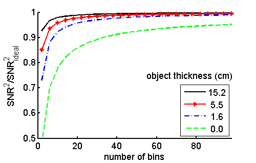
I wrote Matlab code to compute the SNR as a function of the number of PHA bins. I normalized the result by dividing by the ideal, full-spectrum SNR. I also computed the results as a function of object thickness. Recall that the A-vectors for this kind of object lie along a straight line in the A-plane. The results are shown in Fig. 2↓.
Conclusions
There are two interesting features of Fig. 2↑. First, as we expected, the SNR approaches the ideal result as the number of bins gets larger. This is shown mathematically in my paper using the mean value theorem. The second interesting aspect is that the performance with a small number of bins depends strongly on the object thickness. My interpretation of this result is that as the object thickness increases the spectral width also decreases due to beam hardening. Therefore, there is less energy information and it is easier for a low energy-resolution detector to extract it. The improvement occurs for relatively thin objects. From the figure, the three-bin SNR with a 5.5 cm object is about 93% of the ideal value.
Last edited May 12, 2012
© 2012 by Aprend Technology and Robert E. Alvarez
Linking is allowed but reposting or mirroring is expressly forbidden.
References
[1] : Fundamentals of Statistical Signal Processing, Volume I: Estimation Theory . Prentice Hall PTR, 1993.
[2] : Parameter Estimation for Scientists and Engineers. Wiley-Interscience, 2007.