aprendtech.com >> blog >> this post

If you have trouble viewing this, try the pdf of this post. You can download the code used to produce the figures in this post.

A-space covariance from x-ray detector noise

My last post showed that detection performance is determined by the signal to noise ratio (SNR). I derived a formula for the SNR with multispectral measurements, which depends on the covariance of the A-space data. This post shows how to compute the A-space covariance from the x-ray data noise and the effective attenuation coefficient matrix. In general, this depends on the type of estimator used so instead I will use the Cramèr-Rao lower bound (CRLB), which is the minimum covariance for any unbiased estimator. This gives a general result independent of the specific estimator implementation. I will show that the constant covariance CRLB is sufficiently accurate for our purposes. These results will allow us to compute signal to noise ratios for limited energy resolution measurements that are directly comparable to the Tapiovaara-Wagner[3] optimal SNR with complete energy information.

Maximum likelihood estimator with scalar normal data

In a previous post I showed that we could use a linearized model for the transmitted x-ray data

(1) δL_{with_noise} = MδA + w

where L = − log(^I⁄_I₀) is the log of the transmitted flux I , I₀ is the transmitted flux with no object in the beam, M = (∂L)/(∂A) is the gradient of the measurements in A-space, and w is a zero-mean multinormal random variable. Eq. 1↑ is linearized about an operating point (L_o, A_o) so δL = L − L_o and δA = A − A_o. To understand the estimator, I will start by assuming scalar data. The linearized model is then ( I will drop the δ to simplify notation so δL → L and δA → A and the model is assumed to be used around the operating point)

(2) L = MA + w

where w ~ N(0, σ²_L). Since there is only one measurement, a reasonable way to proceed is to solve the deterministic part of (2↑) with the measurement so Â = ^L⁄_M. The variance of the estimate will then be var(Â) = var(w ⁄ M) = ^σ²_L⁄_M².

This estimator is actually the maximum likelihood estimator (MLE). To see this, introduce the log-likelihood function ℒ, which is the logarithm of the probability distribution function evaluated with the actual measurement. The log-likelihood is a function of the data and the unknown parameter ℒ = ℒ(x;A). The maximum likelihood estimator chooses the value of A that maximizes the log-likelihood Â = max[ℒ(x;A)]_A. With scalar normal data, the log-likelihood is

(3) ℒ = − ((L − MA)²)/(2σ²_L) + constant

Notice this reaches its maximum value when the first term is zero. Solving L − MA = 0, the estimator is Â_MLE = ^L⁄_M, which is the solution of the non-random part of the model with the measurement.

The error in the estimate will be proportional to the radius of curvature ρ of ℒ at the maximum value. This is the negative of the second derivative evaluated at A = Â

radius of curvature = ρ = − ⎡⎣(∂²ℒ)/(∂A²)⎤⎦_Â

Differentiating (3↑), the radius of curvature is

ρ = (M²)/(σ²_L)

Notice that we can express the variance of the estimate as the inverse of the second derivative

var(Â) = (σ²_L)/(M²) = (1)/(ρ) = − (1)/(⎡⎣(∂²ℒ)/(∂A²)⎤⎦_Â)

In general, the second derivative may depend on the data, so we would use the expected value of the second derivative

var(Â) = − (1)/(⟨⎡⎣(∂²ℒ)/(∂A²)⎤⎦_Â⟩)

Appendix 3A of Kay[2] proves that this is the minimum variance for any unbiased estimator, called the Cramèr-Rao lower bound (CRLB).

The MLE is the value of the parameter where the derivative is equal to zero. The first derivative of ℒ is

(4) (∂ℒ)/(∂A) = (M)/(σ²_L)(L − MA) = (M²)/(σ²_L)⎛⎝(L)/(M) − A⎞⎠ = I(g(L) − A)

With this factoring, the maximum likelihood estimate is Â_MLE = g(L) = ^L⁄_M. Notice that the variance of the estimate, from my discussion in the first paragraph of this section is var(Â) = (σ²_L)/(M²) = ¹⁄_I . The proof in Appendix 3A of Kay[2] shows that this is a general result. If we can factor the derivative as in (4↑), then the inverse of the leading factor, I , is the CRLB.

Maximum likelihood estimator with vector multinormal data, constant covariance

We can parallel this derivation with vector data by following the two-step approach used in my previous post to derive the optimal detector: first solve the problem assuming “white” equal variance data and then use the whitening transform to convert the general case to the simplified one. If the covariance of the measured data is C_L = σ²_LI, where I is the identity matrix with ones on its diagonal, then the log-likelihood function is

ℒ(L;A) = (1)/(2σ²_L)(L − MA)^T(L − MA) + constant

Expanding the product and gathering common terms utilizing the fact that ℒ is a scalar so we can take the transpose of any term without affecting the result

ℒ(L;A) = (1)/(2σ²_L)[L^TL − 2L^TMA − A^T(M^TM)A] + constant

I will use the general formulas for matrix derivatives from my post,

(∂b^Tx)/(∂x) = (∂x^Tb)/(∂x) = b

(5) (∂x^TBx)/(∂x) = (B + B^T)x = 2 Bx if B symmetric

where b is a constant vector and B is a constant matrix and x is the vector of variables. The derivative of ℒ is (since (M^TM) is symmetric)

(6) (∂ℒ)/(∂A) = (1)/(σ²_L)[M^TL − (M^TM)A] = ((M^TM))/(σ²_L)[(M^TM)^− 1M^TL − A]

The MLE is derived by setting the derivative (6↑) equal to zero so

Â_MLE = (M^TM)^− 1M^TL

and by analogy to the scalar case, the covariance of the estimate is the inverse of the leading factor of (6↑)

cov(Â_MLE) = σ²_L(M^TM)^− 1

We can use these results for the case with a general covariance matrix C_L by using the whitening transform V defined so that C^− 1_L = V^TV and C_L = V^− 1V^− T. Transforming the measurement data so L’ = VL, the transformed linear model is

L’ = V(MA + w) = M’A + w’

where M’ = VM and w’ = Vw. The covariance of w’is the identity matrix

cov(w’) = ⟨(Vw)(Vw)^T⟩ = VC_LV^T = VV^− 1V^− TV^T = I

so we can apply the white case results. Using the MLE from the white case and noting that M’^TM’ = M^TV^TVM = M^TC^− 1_LM

(7) Â_MLE = (M^TC^− 1_LM)^− 1 M^TV^TVL = (M^TC^− 1_LM)^− 1 M^TC^− 1_LL

Similarly, the covariance of the estimate is

(8) cov(Â_MLE) = (M’^TM’)^− 1 = (M^TC^− 1_LM)^− 1

Simple vector MLE example

We can see how these formulas work an example. Suppose we have two-spectrum data such as from two x-ray tube voltages or two bin PHA. In this case the M matrix is

M = ⎡⎢⎣ M₁₁ M₁₂ M₂₁ M₂₂ ⎤⎥⎦

and the covariance is

C_L = ⎡⎢⎣ ¹⁄_N₁ 0 0 ¹⁄_N₂ ⎤⎥⎦

where N₁ and N₂ are the mean values of the photon numbers of the measurements.

Substituting these into (7↑), the MLE is

(9) Â_MLE = (1)/((M₁₁M₂₂ − M₁₂M₂₁))⎡⎢⎣ M₂₂L₁ − M₁₂L₂ − M₂₁L₁ + M₁₁L₂ ⎤⎥⎦

Notice the MLE is just the solution of the linear system MA = L. For example, we can write the solution for A₁̂ using determinants and cofactors as in elementary algebra

A₁̂ = (||| L₁ M₁₂ L₂ M₂₂ |||)/(| M|) = (M₂₂L₁ − M₁₂L₂)/(| M|)

where | | is the determinant.

The covariance of the estimate is

(10) cov(Â_MLE) = (||| (M²₂₂)/(N₁) + (M²₁₂)/(N₂) − ⎛⎝(M₂₁M₂₂)/(N₁) + (M₁₁M₁₂)/(N₂)⎞⎠ − ⎛⎝(M₂₁M₂₂)/(N₁) + (M₁₁M₁₂)/(N₂)⎞⎠ (M²₂₁)/(N₁) + (M²₁₁)/(N₂) |||)/(| M|²)

These results parallel those I derived in my dissertation and my 1976 paper[1]. The covariance (10↑) is Eqs. 14 and 15 of my paper and the MLE (9↑) with two spectra is just the solution of the deterministic equations with the measured data as I showed in my paper.

The matrix multiplications can get tedious so in my next post I will describe how to use the free symbolic mathematics program Maxima to carry them out. I am including Maxima scripts for some of the derivations in the code for this post.

CRLB with general multinormal data

We know that with x-ray data the covariance is not constant. Indeed, the variance increases strongly with object thickness. So an immediate question is: What is the difference between the CRLB computed using constant covariance and the general result that takes the change into account? To answer this, I did a simulation that computes the error by using the constant covariance formula as a function of object thickness.

Appendix 3.C of Kay[2] derives the inverse of the CRLB I(A) for the general multinormal case where the covariance can change. The results are (translated to my notation)

(11) [I(A)]_ij = ⎡⎣(∂L(A))/(∂A_i)⎤⎦^TC^− 1(A)⎡⎣(∂L(A))/(∂A_j)⎤⎦ + (1)/(2)tr⎡⎣C^− 1(A)(∂C)/(∂A_i)C^− 1(A)(∂C)/(∂A_j)⎤⎦

Recall from my derivation of the linearized model that (∂L(A))/(∂A) = M, so this is

[I(A)]_ij = M(:, i)^TC^− 1M(:, j) + (1)/(2)tr⎡⎣C^− 1(A)(∂C)/(∂A_i)C^− 1(A)(∂C)/(∂A_j)⎤⎦

where the notation M(:, k) is the k’th column of M. Comparing this with Eq. 8↑, the first term is the constant covariance CRLB and the second term measures the effect of changes in C as a function of A.

We can see that the constant covariance term in (11↑) will be much larger than the second term as follows. With Poisson data, the variance of the logarithm is the inverse of the expected value and, since the PHA counts are independent, the covariance and its inverse are

C = ⎡⎢⎢⎢⎣ 1 ⁄ N₁ ⋱ 1 ⁄ N_nbins ⎤⎥⎥⎥⎦, C^− 1 = ⎡⎢⎢⎢⎣ N₁ ⋱ N_nbins ⎤⎥⎥⎥⎦,

where N_k is the number of counts in bin k and nbins is the number of bins. The first term in (11↑) is therefore proportional to the number of photons while the second term is essentially the product of C and its inverse and is approximately constant. Since in medical imaging the number of counts is usually large, we would expect that the constant covariance CRLB is much larger than the derivative of the covariance term.

This is shown by the code for this post. The code has Matlab functions to compute the general and constant covariance CRLB for points along a diagonal line through A-space. In order to compute the general CRLB, we need to have formulas for the derivatives of the covariance in (11↑). Since C is diagonal, we only need the derivative of each diagonal element

(12) (∂)/(∂A_i)⎛⎝(1)/(N_k)⎞⎠ = − (1)/(N²_k)(∂N_k)/(∂A_i) = − (M_ki)/(N_k),

which can be computed at each point from M and N_k.

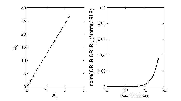
The path through A-space is shown in the left panel of Fig. 1↓. The right panel shows the norm of the difference of the constant covariance and general CRLB matrices divided by the norm of the general CRLB as a function of distance along the line.

Figure 1 Errors with constant covariance CRLB vs object thickness. The object A-vectors lie along a diagonal line through A-space as shown in the left panel. The difference between the general and the constant covariance CRLB divided by the general formula is shown in the right panel.

Conclusions

Fig. 1↑ shows that the errors in the CRLB using the constant covariance formula Eq. 8↑ are less than a few percent although, as expected, they become larger for thicker objects where the number of transmitted photons is smaller. We can therefore use the simpler formula Eq. 8↑ to compute the CRLB of the A-space data without incurring a significant error. Substituting in the formula from my last post, the overall SNR² is

SNR² = δA^TC^− 1_AδA = δA^TM^TC^− 1_LMδA

In the next posts, I will discuss computing the covariance of the measurements for different types of detectors. These require the derivation of the effective attenuation coefficient matrix M and the covariance of the log data C_L. Both of these depend on the properties of the detector and the energy resolution of the measurements. The derivations sometimes involve complex matrix computations, so I double-check them using Maxima and also Monte Carlo simulations.

Bob Alvarez

Last edited Sep 24, 2013

Linking is allowed but reposting or mirroring is expressly forbidden.

References

[1] R. E Alvarez, A. Macovski: “Energy-selective reconstructions in X-ray computerized tomography”, Phys. Med. Biol., pp. 733—44, 1976.

[2] Steven M. Kay: Fundamentals of Statistical Signal Processing, Volume I: Estimation Theory . Prentice Hall PTR, 1993.

[3] M. J. Tapiovaara, R. Wagner: “SNR and DQE analysis of broad spectrum X-ray imaging”, Phys. Med. Biol., pp. 519—529, 1985.