aprendtech.com >> blog >> this post

If you have trouble viewing this, try the pdf of this post. You can download the code used to produce the figures in this post.

Detection with multinormal data

In my previous post, I showed that multivariate normal is a good model for x-ray measurements and in my last post I described the general properties of this distribution. In this post, I will discuss statistical detection theory with the normal model. I will show that the performance is characterized by a suitably defined signal to noise ratio. This will enable me to close the loop to the main topic of this series of posts, which is to explain the results in my paper, “Near optimal energy selective x-ray imaging system performance with simple detectors[1]”, which is available for free download here.

Section 3.3 of Kay[2] has an excellent discussion of classical statistical detection theory and Sec. 2.6 of Van Trees[4] describes its use with normal distributed data. I recommend that you study these references. Here, I will summarize and tie together their results. The main result will be that the probability of detection for a specified false alarm rate depends only on the signal to noise ratio (SNR) and the derivation of the SNR for vector data.

Binary decision making with mean-shifted data

Statistical detection theory is based on hypothesis testing. The simple binary hypothesis testing approach that I will use assumes that the probability distribution functions under both hypotheses are known. The problem is to decide between the hypotheses based on the random measurement(s). In my discussion, I will focus on the multinormal distribution with the same covariance under both hypotheses. With x-ray measurements, we know that the variance depends on the number of photons, which varies strongly with object thickness. This would seem to imply that the analysis is only applicable for thin features. In a future post, I will show that this is not necessarily true but the thin feature case is important since the objects significant for medical diagnosis like lung nodules or breast tumors are many times small. The equal covariance case is also widely used since it provides good insight to the factors affecting detection performance.

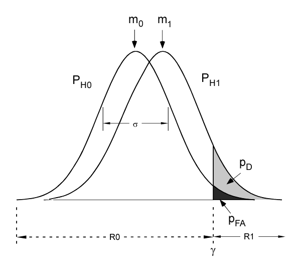
Suppose, we make just one measurement and the distributions P_H₀ and P_H₁ under the two hypotheses have the same variance σ with means m₀ and m₁ as shown in Fig. 1↓. To implement the detection algorithm, we divide the x-axis into two regions and decide H₀ if the measurement is in R₀ and H₁ in R₁. Because of the random data, we cannot eliminate errors. We can measure the performance by two parameters, the probability of detection, P_D = Prob(H₁;H₁) and the probability of false alarm, P_FA = Prob(H₁;H₀), where the notation Prob(H_i;H_j) means the probability of deciding H_i if H_j is true. Since m₀ is less than m₁ for the case shown in Fig. 1↓, a reasonable decision rule is to choose H₀ if x is less than a threshold γ and H₁ if it is larger. The equal case has zero probability so it can be assigned to either case. This leads to the decision regions R₀ and R₁ shown in the figure.

Figure 1 Hypothesis testing with a single measurement

The Neyman-Pearson (NP) theorem

Given the data in Fig. 1↑, an immediate question is where to set the threshold. We cannot simultaneously minimize P_FA and maximize P_D but we can fix P_FA at some pre-determined value α and maximize P_D by using the Neyman-Pearson theorem

To maximize P_D for a givenP_FA = α, decide H₁ if
(1) R(x) = (p(x;H₁))/(p(x;H₀)) > τ

where the parameter τ is chosen so
P_FA = ⌠⌡_{{x;R(x) > τ}}p(x;H₀)dx = α

Note that the theorem is applicable to vector as well as scalar data.

Applying the NP theorem to scalar data

The probability distribution functions (PDF’s) under the two hypotheses are

(2) p(x;H_k) = (1)/(√(2πσ²))exp⎡⎣ − (1)/(2)⎛⎝(x − m_k)/(σ)⎞⎠²⎤⎦ k = 1, 2

Taking the logarithm of the likelihood ratio R in (1↑), substituting the PDF’s (2↑) and changing the variable to u = x − m₀, the NP test is

ℒ(u) = logR = (u² − (u − δm)²)/(2σ²) > logτ

Expanding the left side and rearranging terms, the NP test is u > γ’ where

(3) γ’ = (σ²logτ)/(δm) + (δm)/(2)

With these, we can compute the optimal probability of detection for a specified false alarm rate. First, I will define some notation. Let F(x) be the cumulative distribution function of the N(0, 1) random variable

F(x) = (1)/(√(2π))^x⌠⌡_− ∞e^{− (t²)/(2)}dt

and F_c = 1 − F be its complement. Since u has an N(0, σ²) distribution

P_FA = F_c⎛⎝(γ’)/(σ)⎞⎠

We can invert this since F_c is a monotonically decreasing function so γ’ = σF^− 1_c(P_FA). Since p(x;H₁) ~ N(δm, σ²), the probability of detection is

P_D = F_c⎛⎝(γ’ − δm)/(σ)⎞⎠

Substituting for γ’,

(4) P_D = F_c⎛⎝F^− 1_c(P_FA) − (δm)/(σ)⎞⎠

This shows that the probability of detection for a given false alarm probability depends only on the signal to noise ratio (or its square)

(5) SNR² = ((⟨x;H₁⟩ − ⟨x;H₀⟩)²)/(variance(x;H₀))

where ⟨x;H_k⟩ denotes the expected value of x with the p(x;H_k) distribution.

We can evaluate Eq. 4↑ using Matlab functions to evaluate F_c, andF^− 1_c . The Matlab function normcdf computes F and F_c = 1 − normcdf. Also, the Matlab norminv function computes F^− 1 and F(F^− 1(x)) = x = 1 − F_c(F^− 1(x)) so

F_c(F^− 1(x)) = 1 − x F^− 1(x) = F^− 1_c(1 − x)

Setting t = 1 − x,

F^− 1_c(t) = norminv(1 − t)

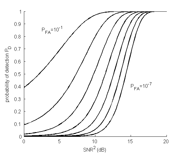
Fig. 2↓ shows the probability of detection P_D as a function of the SNR² in decibels (dB) for different values of the false alarm probability P_FA. Note that as expected, P_D always increases as the signal to noise ratio increases. The code to reproduce this figure is available here. This figure should be compared with Fig. 3.5 of Kay[2].

Figure 2 P_D as a function of signal to noise ratio squared.

Binary decisions with vector data: the equal covariance case

With multivariate normal data and assuming equal covariance under the two hypotheses, the probability distributions are (see my last post).

p(x;H_k) = (1)/((2π)^ⁿ⁄₂| C|^¹⁄₂)exp[ − ¹⁄₂( x − m_k)^TC^− 1(x − m_k)] k = 1, 2

where C is the covariance and n is the dimension of the vector data. Substituting in the definition of the likelihood ratio (1↑) and taking the logarithm of both sides, the log-likelihood is

ℒ(x) = − ((x − m₁)^TC^− 1(x − m₁) − (x − m₀)^TC^− 1(x − m₀))/(2)

Expanding the products, gathering terms, and defining δm = m₁ − m₀

− 2ℒ(x) = δm^TC^− 1x + m^T₁C^− 1m₁ − m^T₀C^− 1m₀

The last two terms on the right hand side do not depend on the data and a multiplicative factor does not not affect the results so the Neyman-Pearson test is

(6) ℒ(x) = δm^TC^− 1x > γ’

The log-likelihood ℒ(x) is a linear combination of a multivariate normal random variable so it also has normal distribution. It is a scalar so we can apply the results of the previous section to see that the performance is determined by the SNR² from Eq. 5↑

(7) SNR² = ((⟨ℒ;H₁⟩ − ⟨ℒ;H₀⟩)²)/(variance(ℒ;H₀))

From (6↑), the expected values are

(8) ⟨ℒ;H_k⟩ = δm^TC^− 1m_k

so the numerator of (7↑) is

(9) (⟨ℒ;H₁⟩ − ⟨ℒ;H₀⟩)² = ( δm^TC^− 1δm)²

Using the definition of variance

(10) variance(ℒ;H₀) = ⟨(ℒ(x) − ⟨ℒ;H₀⟩)^T(ℒ(x) − ⟨ℒ;H₀⟩)⟩

From the definition of ℒ (6↑) and the expected value (8↑),

ℒ(x) − ⟨ℒ;H₀⟩ = δm^TC^− 1(x − m₀) = (x − m₀)^TC^− 1δm

where the last step follows because ℒ is a scalar so it is equal to its transpose as is the covariance because it is symmetric.

(11) variance(ℒ;H₀) = ⟨ δm^TC^− 1(x − m₀)(x − m₀)^TC^− 1δm⟩ = δm^TC^− 1CC^− 1δm = δm^TC^− 1δm

Substituting (9↑) and (11↑) in (7↑), the vector SNR² is

(12) SNR² = δm^TC^− 1δm

Example: “white” data

Data with independent, equal variance provide good insight and are also important in practice since we can use the whitening matrix, Φ_w discussed in my last post, to transform any multinormal to this case. In a future post, I will describe how we can use whitening with x-ray spectral data.

For whitened data, the covariance matrix is C = σ² I and its inverse is C^− 1 = ¹⁄_σ² I. Substituting in (12↑), the signal to noise ratio is

SNR²_W = (|δm|²)/(σ²)

This is the distance between the means squared divided by the variance. From (6↑), the NP test is

ℒ(x) = (1)/(σ²) δm^Tx > γ’

This is the dot product of the data with the mean difference vector δm.

Conclusion

I have now provided the statistical detection theory framework that I will use to analyze the Tapiovaara-Wagner imaging task[3] for x-ray data with spectral information. We can use this framework to introduce the basis set expansion of the attenuation coefficient as shown in my paper[1]. This will allow us to compare the performance of systems with limited energy resolution to the ideal case with full spectral information.

Bob Alvarez

Last edited Jan 20, 2012

Linking is allowed but reposting or mirroring is expressly forbidden.

References

[1] Robert E. Alvarez: “Near optimal energy selective x-ray imaging system performance with simple detectors”, Med. Phys., pp. 822—841, 2010.

[2] Steven M. Kay: Fundamentals of Statistical Signal Processing, Volume 2: Detection Theory. Prentice Hall PTR, 1998.

[3] M. J. Tapiovaara, R. Wagner: “SNR and DQE analysis of broad spectrum X-ray imaging”, Phys. Med. Biol., pp. 519—529, 1985.

[4] H. L. Van Trees: Detection, Estimation, and Modulation Theory. Part I: Detection, Estimation, and Linear Modulation Theory. John Wiley & Sons Inc, 2001.