aprendtech.com >> blog >> this post

If you have trouble viewing this, try the pdf of this post. You can download the code used to produce the figures in this post.

SNR with energy information

In the next posts I will discuss some of the results in my recent paper “Near optimal energy selective x-ray imaging system performance with simple detectors[1]”, which is available for free download here. The paper discusses fundamental limits on the signal to noise ratio of x-ray detectors with energy spectrum information. It also describes how we can design practical systems with low energy resolution detectors whose performance gets close to the optimal limit.

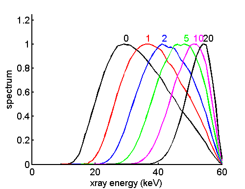
As shown in my previous posts, the energy spectrum changes as x-rays are transmitted through an object and the changes depend on the properties of the object. An example of the change in spectrum is shown in Fig. 1↓, which plots the normalized spectrum for different object thicknesses. The increase in the average energy with thickness is called beam hardening. A detector that does not measure the spectral changes is not extracting all the available information. It will therefore have a poorer signal to noise ratio (SNR) than one that does. In this post, I will show that there is a maximum SNR that can be achieved by systems that measure the complete spectrum of the x-rays transmitted through the object. This limit is extremely useful because it gives us an absolute scale to compare the performance of real systems. I derive expressions for the SNR of photon counting and energy integrating systems and show that they are less than the optimal SNR whenever the incident spectrum has non-zero width. If the spectrum has zero width, then there is no energy spectrum information available for the detector to extract and all the detector types have the same SNR.

In addition to my paper, the discussion is based on the paper “SNR and DQE analysis of broad spectrum x-ray imaging” by M. J. Tapiovaara and R. Wagner[4] and also papers by Cahn et al.[2] and Giersch et al.[3].

Imaging task and SNR

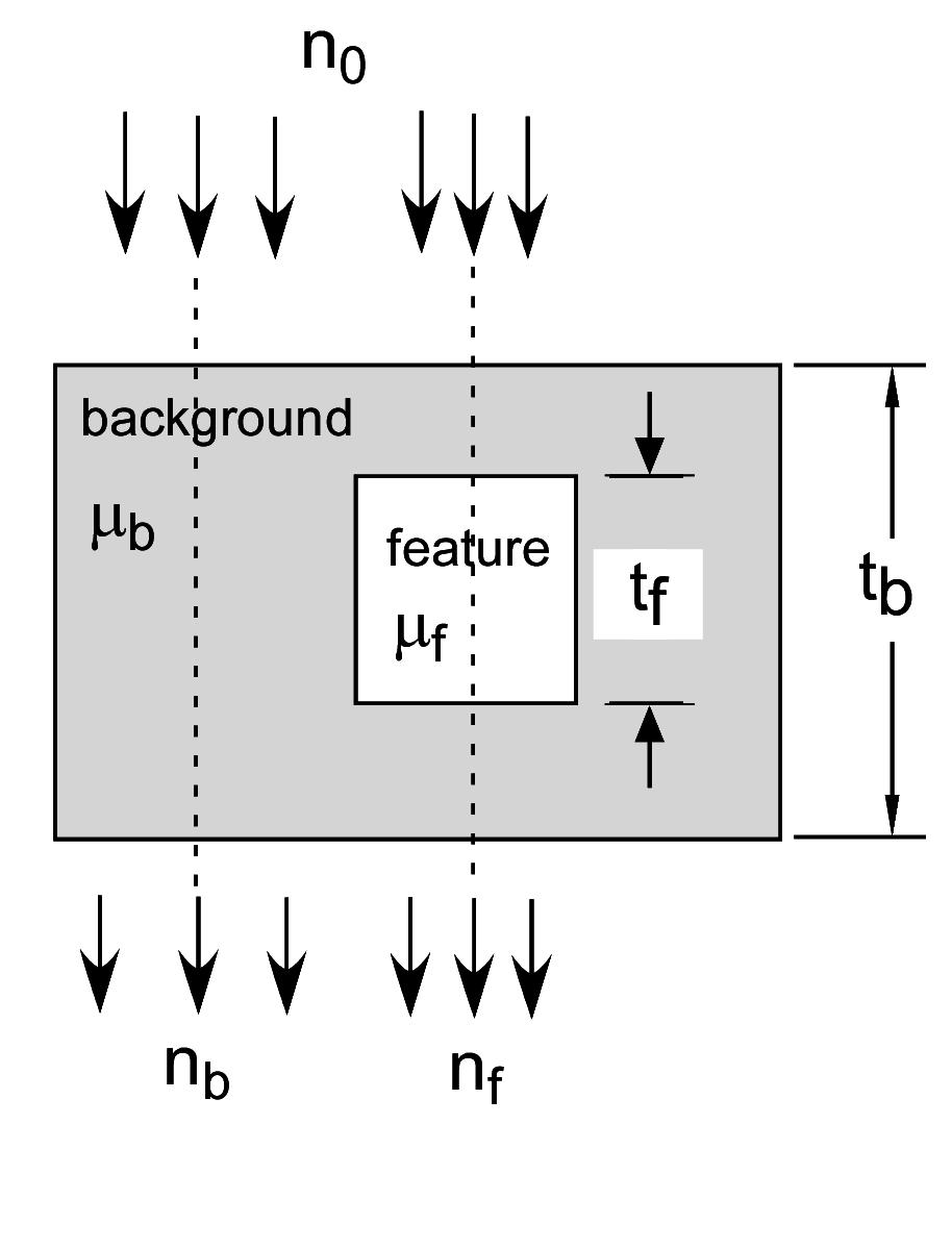
We need a model for both the signal and the noise to define SNR . The definition of the signal requires an imaging task, which I show in Fig. 2↓. The task is to detect a feature embedded in a background from measurements of the transmitted photons in the background n_b(E) and the feature n_f(E) region. The measurements are specified by the photon number spectra so n(E)dE is the number of photons in the range from E to E + dE. In this post, I will assume that we have perfect energy spectrum measurements with an infinite number of PHA bins of infinitesimal width. I will also assume the deadtime is zero so n(E)dE is a Poisson random variable and measurements in non-overlapping energy regions are independent.

Figure 1 Change in spectrum vs. the object thickness.

For this imaging task, the signal is the expected value of the difference of the integrated measurements in the two regions N_f = ∫n_f(E)dE and N_b = ∫n_b(E)dE. Since the expected value of a sum is the sum of the expected values

⟨N⟩ = ⌠⌡⟨n(E)dE⟩ = ⌠⌡n(E)dE

where the non-bold symbol is the expected value ⟨n(E)⟩ = n(E). Therefore the signal is

Signal = ⌠⌡(n_f(E) − n_b(E))dE.

Since we have complete spectrum information, we can weight the spectrum with a function w(E) when we calculate the signal resulting in

Signal = ⌠⌡(n_f(E) − n_b(E))w(E)dE.

Figure 2 Imaging task for SNR computation.

With my idealized assumptions, the signals in non-overlapping energy intervals are Poisson distributed and independent. Since the variance of a Poisson is equal to the expected value, the signal variance is

Variance = ⌠⌡(n_f(E) + n_b(E))w²(E)dE

where I have used the fact that the variance of a weighted sum of independent random variables is the sum of square of the coefficients times the variances of the variables. The SNR squared is then

(1) SNR² = ([⌠⌡(n_f(E) − n_b(E))w(E)dE]²)/(⌠⌡(n_f(E) + n_b(E))w²(E)dE)

Optimal SNR

The numerator of Eq. 1↑ is an inner product integral, which is analogous to the ordinary dot product of two vectors a⋅b. Since a⋅b = |a||b|cos(θ), where θ is the angle between the vectors, |a| = √(a⋅a), |b| = √(b⋅b), and 0 ≤ cos²(θ) ≤ 1, we can square both sides of the equation to show

(a⋅b)² = ( a⋅a)(b⋅b)cos²(θ) ≤ (a⋅a)(b⋅b).

The equality is only when a and b are parallel, that is a = Cb, where C is a scalar. The analogous relation for the inner product of functions is the Schwartz inequality

(2) [⌠⌡fgdE]² ≤ (⌠⌡f²dE)(⌠⌡g²dE)

Letting f = w(E)√(n_f(E) + n_b(E)) and g = (n_f(E) − n_b(E)) ⁄ √(n_f(E) + n_b(E)), then

(3) fg = (n_f(E) − n_b(E))w(E)

and

(4) ⌠⌡f²dE = ⌠⌡(n_f(E) + n_b(E))w²(E)dE

(5) ⌠⌡g²dE = ⌠⌡((n_f(E) − n_b(E))²)/(n_f(E) + n_b(E))dE

Substituting (3↑), (4↑), and (5↑) in (2↑)

[⌠⌡(n_f(E) − n_b(E))w(E)dE]² ≤ [⌠⌡(n_f(E) + n_b(E))w²(E)dE]⎡⎣⌠⌡((n_f(E) − n_b(E))²)/(n_f(E) + n_b(E))dE⎤⎦

Assuming the non-trivial case where the first term in brackets is not zero we can divide through by it and comparing to Eq. 1↑ for SNR²,

(6) SNR² ≤ ⌠⌡((n_f(E) − n_b(E))²)/(n_f(E) + n_b(E))dE.

The optimal SNR can be achieved when f = Cg, where C is a constant. This can be done by letting the weighting function equal

(7) w(E) = C(n_f(E) − n_b(E))/(n_f(E) + n_b(E))

Low contrast object approximation

We can get some insight into these equations by analyzing the low contrast feature case. If the spectrum incident on the object is n₀, then

n_b = n₀e^{− μ_bt_b}

n_f = n₀e^{− μ_b(t_b − t_f) − μ_ft_f} = n_be^{− (μ_f − μ_b)t_f}

Letting δμ = μ_f − μ_b , with a low contrast feature, (δμ)t_f≪1. Then

(8) n_f − n_b = (e^{− δμ t_f} − 1)n_b ≈ − δμ t_fn_b.

Also

(9) n_f + n_b ≈ 2n_b

Substituting these in the equation for the SNR², (1↑)

(10) SNR² ≈ t²_f([⌠⌡w(E)n_b(E)δμ(E)dE]²)/(2⌠⌡w²(E)n_b(E)dE)

Photon counting and energy integrating SNR

We can use Eq. 10↑ to analyze three important cases: 1. a photon counting detector, 2. an energy integrating detector, and 3. the optimal detector with complete energy spectrum information. The photon counting detector counts all photons regardless of their energy, so w(E) = 1. The total photons transmitted through the object is λ = ∫n_b(E)dE and the normalized transmitted spectrum is n̂_b = n_b ⁄ λ. Using these, the SNR² of the photon counting detector in the low contrast approximation is

(11) SNR²_{photon counting} = (λt²_f)/(2)[⌠⌡n̂_b(E)δμ(E)dE]² = λt²_f⟨δμ⟩²_N ⁄ 2

where ⟨δμ⟩_N is the effective value of δμ in the transmitted photon number spectrum.

Next, we can analyze the energy integrating detector. This detector sums the energies of the photons, so it weights photons according to their energy w(E) = E. Rewriting the low contrast SNR Eq. 10↑ in terms of n̂_b,

SNR² = λt²_f([⌠⌡w(E)n̂_b(E)δμ(E)dE]²)/(2⌠⌡w²(E)n̂_b(E)dE).

Substituting w(E) = E, we can write this equation in terms of the normalized energy spectrum

q̂(E) = (En̂_b(E))/(⌠⌡En̂_b(E)dE).

Noting that ∫En̂_b(E)dE = ⟨E⟩ is the effective energy and ∫E²n̂_b(E)dE = ⟨E²⟩ is the effective energy squared, the SNR of the energy integrating detector is

SNR²_{energy integrating} = λt²_f([⌠⌡En̂_b(E)δμ(E)dE]²)/(2⌠⌡E²(E)n̂_b(E)dE) = λt²_f(⟨E⟩²⟨δμ⟩²_Q)/(2⟨E²⟩)

Defining the excess variance

F = (⟨E²⟩)/(⟨E⟩²)

(12) SNR²_{energy integrating} = λt²_f⟨δμ⟩²_Q ⁄ 2F

Comparing this with the SNR of the photon counting detector, Eq. 11↑, we can see that the energy integrating SNR is smaller for two reasons. First, since the energy spectrum q(E) = En(E), it has a larger effective energy than the photon number spectrum. Since attenuation coefficients in the medical x-ray energy range decrease with energy, ⟨δμ⟩²_Q < ⟨δμ⟩²_N. Also, we can use the computational formula for the variance, var(X) = ⟨X²⟩ − ⟨X⟩², to see that ⟨E²⟩ ≥ ⟨E⟩² since the variance is always non-negative. Therefore F ≥ 1. The equal case occurs if the incident spectrum is zero width, that is we have no energy information. So,

SNR²_{photon counting} ≥ SNR²_{energy integrating}.

Optimal SNR and weighting function for low contrast object

We can substitute the low contrast object equations for n_f − n_b (Eq. 8↑) and n_f + n_b (Eq. 9↑) in the equation for the optimal SNR (6↑) with complete energy information (6↑) to show that

SNR²_optimal = ⌠⌡((n_f(E) − n_b(E))²)/(n_f(E) + n_b(E))dE = ⌠⌡([δμ t_fn_b]²)/(2n_b)dE = λt²_f⟨δμ²⟩_N ⁄ 2

By the same argument I used with F, ⟨δμ²⟩_N ≥ ⟨δμ⟩²_N so

SNR²_optimal ≥ SNR²_{photon counting} ≥ SNR²_{energy integrating}

with the SNR being equal only with zero width spectra that provide no energy information.

The optimal weighting function in the low contrast case is also interesting. Again substituting the equations for the sums and differences of n_f and n_b in the general formula (7↑)

w(E) = C(n_f(E) − n_b(E))/(n_f(E) + n_b(E)) = − Ct_fδμ ~ δμ

That is, the optimal weighting function is proportional to the difference of the attenuation coefficients. By my discussion of attenuation coefficients, they can be approximated by a two-function basis set. One possibility is the Compton scattering/photoelectric basis set. The Compton part does not vary much with energy and depends on electron density, so it is approximately the same for all biological materials. The difference of the attenuation coefficients is mainly the photoelectric interaction, which varies the inverse of the cube of energy 1 ⁄ E³. The optimal weighting function decreases rapidly with energy. Notice that this is the opposite of the energy integrating weighting function, which is proportional to energy.

Discussion

The optimal SNR provides a useful yardstick to gauge the performance of imaging systems that is closely related to detective quantum efficiency (DQE). However, my discussion so far assumes that we measure the full, high-resolution energy spectrum. Since we know that the quantity being measured, the attenuation coefficient, is a smooth low-dimensionality function, it may be possible to achieve close to optimal SNR with low-resolution measurements. That was the principal subject of my paper[1] and I will discuss it in the following posts. My next describes a Monte Carlo simulation of the theoretical results in this post.

--Bob Alvarez

Last edited Aug 07, 2019

Linking is allowed but reposting or mirroring is expressly forbidden.

References

[1] Robert E. Alvarez: “Near optimal energy selective x-ray imaging system performance with simple detectors”, Med. Phys., pp. 822—841, 2010. URL http://tinyurl.com/NearOptimalEnergySelective.

[2] R N Cahn, B Cederström, M Danielsson, A Hall, M Lundqvist, D Nygren: “Detective quantum efficiency dependence on x-ray energy weighting in mammography”, Med. Phys., pp. 2680—2683, 1999.

[3] Jorgen Giersch, Daniel Niederlohner, Gisela Anton: “The influence of energy weighting on X-ray imaging quality”, Nucl. Instrum. Methods A, pp. 68—74, 2004.

[4] M. J. Tapiovaara, R. Wagner: “SNR and DQE analysis of broad spectrum X-ray imaging”, Phys. Med. Biol., pp. 519—529, 1985. URL http://doi.org/10.1088/0031-9155/30/6/002.