If you have trouble viewing this, try the pdf of this post. You can download the code used to produce the figures in this post.
Logarithm of PHA with deadtime
The logarithm of the data is often used in x-ray imaging systems because it is (very) approximately proportional to the line integral. The statistics of the log of the counts in photon counting detectors are are different than those of the counts as summarized in my last post and I derive them in this post. I then test the formulas using a Monte Carlo simulation.
General formulas for expected value, variance, and covariance of log of counts
With a counting detector, the logarithm is mathematically ill-defined because the counts can have a value of zero. In hardware implementations, a value of one is usually added to the data. This does not affect the rersults because typically the counts are much greater than one. Here, I will assume that this has been done so the logarithm of the data is mathematically well behaved.
Suppose we have a random variable X and we want to derive expressions for the mean and variance of Y = log(X). We can use a general result[1] based on a series expansion of a function y = g(x) about the expected value λ = ⟨X⟩
(1) g(x) = g(λ) + g’(λ)(x − λ) + g’’(λ)((x − λ)2)/(2) + …
Using this series,
⟨g(X)⟩ ≈ g(λ) + g’’(λ)(σ2x)/(2)
var[g(X)] ≈ [g’(λ)]2σ2x
If g(x) = log(x) then g’(x) = (1)/(x) and g’’(x) = − (1)/(x2). Combining these results with those of the previous section gives the following for the log random variable log(X)
var[log(X)] ≈ (σ2x)/(λ2)
For counting variables that are approximately Poisson distributed, σ2x ≈ λ and λ≫1, so the second term in Eq. 2↑ is much smaller than the first and
We also require the covariance. Using the identity cov(X, Y) = ⟨XY⟩ − ⟨X⟩⟨Y⟩,
To evaluate the first term in (4↑), we can use
log(X) = log⎡⎣⟨X⟩⎛⎝1 + (δX)/(⟨X⟩)⎞⎠⎤⎦ ≈ log(⟨X⟩) + (δX)/(⟨X⟩)
with a similar expression for log(Y). With these two expansions, the first term becomes
Substituting Eq. 5↑ in Eq. 4↑ and using the fact that, from Eq. 3↑, for a counting variable, ⟨log(X)⟩ ≈ log(⟨X⟩),
The general formulas for the log variables are summarized in the first table:
| mean value | ⟨log(X)⟩ ≈ log(⟨X⟩) |
| variance | var[log(X)] ≈ (var(X))/(⟨X⟩2) |
| covariance | cov[log(X), log(Y)] ≈ (cov(X, Y))/(⟨X⟩⟨Y⟩) |
while from my last post the formulas for the mean, variance, and covariance of the counts in PHA bins Mk are
| mean value | ⟨Mk⟩ = ⟨M⟩pk |
| variance | var(Mk) = ⟨M⟩pk + (var(M) − ⟨M⟩)p2k |
| covariance | cov(Mj, Mk) = pjpk(var(M) − ⟨M⟩) |
Combining these, we can compute the stats for the logarithm of the PHA bin counts log(Mk).
Monte Carlo simulation
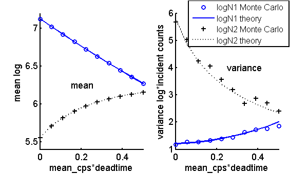
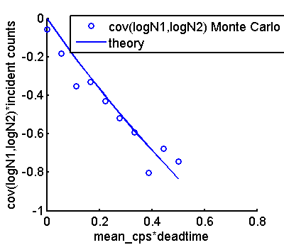
Since the formulas for the log variables are in terms of the count statistics, we can simulate them using a straightforward extension of the code from my last post. The code for this post was used to compare the theoretical formulas and the Monte Carlo results. The mean and variance data are plotted in Fig. 1↓ and the covariance in Fig. 2↓
Discussion
The Monte Carlo results and the theoretical formulas are in good agreement. As I noted previously, the Monte Carlo variance and covariance are noisier than the mean values.
It is worth emphasizing that the changes in the statistics in this and my previous posts is due to differences in the assumed parameters of the detectors. In all cases, the photon numbers and spectrum did not change. This means that in our processing of the data we need to know these parameters and rely on them being constant or having some way to predict them. It is probable that the parameters will be different for different detectors in the same array.
In the early days of CT, differences in detectors were a major problem leading to the dreaded ring artifacts. I spent a lot of time trying to correct these differences and never succeeded completely. In retrospect, I believe that the differences were not only in gain but in the energy spectral response of different channels of an array. Ultimately manufacturers solved this problem mainly by improving the detectors themselves and reducing the inter-channel variations.
I think that with photon counting detectors the improvements will come mainly from improvements in their parameters and much less from algorithms to correct their defects. However, the theory developed here helps us to understand and specify the range and tolerance required for the detectors.
Last edited Dec 05, 2011
© 2011 by Aprend Technology and Robert E. Alvarez
Linking is allowed but reposting or mirroring is expressly forbidden.
References
[1] : Probability, Random Variables, and Stochastic Processes. McGraw-Hill, 1965.