A Matlab interface for a projection simulator for image reconstruction research

edit: Oct. 4, 2011 The C++ code referred to in this post has been superseded by a Matlab only version that is faster and has more geometric shapes. The Matlab function uses the approach described here so it gives similar results.

My last post discussed C++ code for a CT projection simulator. In this post, I will describe a Matlab interface to the simulator executable.

There are several ways this could be done. One is to write a mex interface. But this requires some contortions since mex is basically a standard C interface and the simulator code is written in C++. Besides, mex has some major limitations such as not being backward compatible for previous versions of Matlab. So I will use a quick and dirty implementation where I write out a specification .sct file, execute the simulator using the dos command, and then read the projection data file back into Matlab. I have found that the overhead of this approach is not significant compared to the time to execute the simulator. Also, unix users can probably use the system command but I have not tried it. If anyone is able to run the code on unix, let me know.

The box below shows an example of the use of the function to create the data from my last post.

%% Create projection data   
  % edit the directory in following line for your computer 
workdir = ’E:\Projects\Progutil\CTsim\Debug\’; 
spec_ellipse = [2  -3   2   5  30   1 0.5; ... 
    2  -3   1.5   4.5  30   -1 0.25]; % two ellipses 
spec_circle = [-2 0 4 1 1];
[prj,siz] = ct_proj_parallel(0.1,180,’ellipse’,spec_ellipse,...
   ’circle’,spec_circle,’workdir’,workdir);

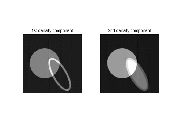
The function uses Matlab double arrays to specify the shapes. The specification arrays have data for each instance of the shape in separate rows. Each specification contains the data for the instance in the order used in the C++ CTsim function. For example, the ellipse specifcation is “x y semi-major semi-minor angle density.” The example above specifies a length- two vector density.

I had to modify the code slightly so I could easily specify the working directory in Matlab. I did this by making the prefix a user specified option with the default being no prefix. Instead of writing out the data with the “sc” prefix, the C++ code overwrites the specification file and adds the “.sdt” file with the projection data. The code includes the input specifications but it does not include the comments so if you are using CTsim.exe from the command line, you should keep a copy of your original file. Of course, it does not matter with ct_proj_parallel.m since the input and output files are written and then erased.

The steps to compile the C++ code are described in my last post.

The reconstructed images of each of the components of the data are shown in Fig. 1↓.

As the name implies, the Matlab function ct_proj_parallel implements a parallel beam projection. The implementation can be extended to implement fan and cone beam projections by modifying the C++ code.

Figure 1 Reconstructed images of each of the components of the projection data.

Last edited July 25, 2011

Linking is allowed but reposting or mirroring is expressly forbidden.

A Matlab interface for a projection simulator for image reconstruction research

References