If you have trouble viewing this, try the pdf of this post. You can download the code used to produce the figures in this post.

My last post discussed the approach for my CT projection simulator. In this post, I will describe the C++ implementation.

In my approach, the object is specified as a set of geometric objects whose parameters are described in a text function that is the input to the program. The attenuation is linear so the final object is the sum of all the component objects. The parameters of each object include the location, size and orientation. In addition, each object has a vector density, which can describe the a-vector in a simulation of energy dependent x-ray attenuation. Of course, the density can also be a scalar by using a vector of length 1. The density of all the component objects must have the same length.

The text file specification has the advantage that it is readable and can be created with any text editor. An example is

There are two kinds of lines—comments and parameters. Comment lines have a ’#’ character in the first column. These are ignored by the software but are useful for humans. Parameter lines start with a ’-’ in the first column. This is followed by a parameter name and a space. The rest of the line is a string specifying the value of the parameter. Note that the specification string can contain any character including spaces and commas. The interpretation of the string is done by the program. Note that the order of the parameters is not important. Duplicate parameters will cause an error.

For obscure historical reasons, I use a ’.sct’ extension for a parameter file so an example would be ’spec.sct.’

In the example above you can see single parameter specifications such as setting ’ntheta’, the number of angles in the projection, to 180. The objects are specified by two parameters. One of the parameters, ’nellipses’ in the example specifies the number of ellipse objects. The program then expects the object specifications in separate lines such as ’ellipse0’. The second ellipse is specified by the ’ellipse1’ parameter line. An ellipse is specified by 6 or more float numbers that are separated by spaces. The first two are the (x,y) coordinates followed by the two semi-major and semi-minor axes of the ellipse. The fifth parameter is the angle in degrees. The rest of numbers specify the density vector. In the example above, the density of ellipse1 is the two length vector [1 0.5]. The density of the second ellipse is [-1 0.25].

A single sphere object is also specified. The parameters are [x_center y_center z_center radius density].

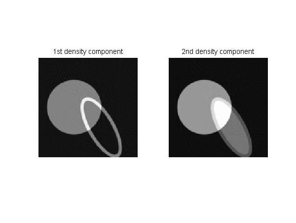
Fig. 1↓ shows the images created by reconstructing the two components of the projection data produced by CTsim using the specification above. The command line is shown in the box. Matlab code to create the figures is included with the code for this post.

The scan geometry is specified by a Gantry object, which is composed of an (x-ray) tube location, a detector, and a rotation angle. The gantry starts at angle 0 with the line detector parallel to the x-axis at a ’detector_distance’ from the origin and the tube on the y axis spaced ’tube_distance’ from the origin. The detector has ’ndetectors’ elements that are spaced with ’detector_spacing’ around the origin. The locations are determined by code analogous to this Matlab snippet. Notice that the center detector is not necessarily at x = 0. Also, all of the dimensions of the gantry and the geometric objects have to be in consistent units.

To generate scan data, the gantry starts at angle 0. Lines from the tube to each of the detector positions are generated and the length of the intersection of each line with the component objects times the object densities are accumulated and stored for each detector and each angle to form the ’sinogram.’ For parallel projections, which are specified by the ’-p’ command line argument to the program, the ’detector_distance’ and ’tube_distance’ parameters are ignored and are not required. The lines are then perpendicular to the detector line and through each detector. The gantry is rotated by rotating the vector of the tube and the detector line around the origin.

Note that the origin for the object should be at its center and not at a corner of the field as would be the case for the object image. This implies that some of the component coordinates will be negative.

The program generates one projection for each component of the density. Note that the components of the density for each object can be different. The vector projections array is output by the program as floating point data. The data are arranged as one row for each sinogram location (in ’C’ standard row-major order for the two dimensional number of angles by number of detectors projections array) and the number of columns equal to the dimension of the density. I use a two file format. One file of type ’.sct’ specifies the array dimensions (ny for number of rows and nx for number of columns) and data type (float) using the same syntax as for the geometry specification. The input geometry specification is also copied to the ’.sct’ file. The other file with a .’sdt’ extension contains the floating point data. The output file name is a ’sc’ prefix and the geometry file name, for example ’scspec.sct’ and ’scspec.sdt’.

edit: July 26, 2011

This prefix causes problem with a filename that includes the path. For example if the specification is “C:\spec.sct”, then “scC:\spec.sct” is not a legitimate file name. So I modified the code to make the prefix optional. The default is no prefix. This allows calling programs to use filenames with paths. However, it overwrites the spec.sct file with information for the projections. The code copies over the data from spec.sct but not the comments so you may want to keep a copy of your original file.

I also modified the Matlab function included with the code package to take this into account.

end edit: July 26, 2011

As one of my colleagues used to say, the ultimate documentation is the code. You will notice that the internal geometry is three dimensional. I have used this framework in the past to generate projections with an area detector. I use a Line object extensively. The object specifies a line using two three-dimensional vectors. The ’n’ vector is a vector from the origin perpendicular to the line. The ’s’ vector has unit length and is parallel to the line.

Windows users can compile the code with the free Microsoft Visual Studio Express 2008 compiler.

Linux and Windows users can also compile with the free CodeBlocks IDE and the gnu C++ compiler.

To test the software, copy the spec.sct file to the directory with the executable. Then, from the command line do

Start Matlab and execute P8ctsim2.m to read in the projections, reconstruct and display them.

In my next post, I will describe a Matlab interface to the projection simulator.

Last edited July 15, 2011

© 2011 by Aprend Technology and Robert E. Alvarez

Linking is allowed but reposting or mirroring is expressly forbidden.

References