A projection simulator for image reconstruction research--rationale

edit: Oct. 4, 2011 The C++ code referred to at the end of this post has been superseded by a Matlab only version that is faster and has more geometric shapes. The Matlab function uses the approach described here so the rationale is still valid.

Simulators are essential tools in CT research. They provide data with known properties to test reconstruction algorithms and simulations of complete systems. Matlab provides simulators with the radon and fanbeam functions of the Image Processing Toolbox. However, these functions specify the object as a raster image, which leads to large artifacts in the projections and in the reconstructed images.

The problem is illustrated in Figs. 1↓ and 2↓. These show reconstructions of the Shepp-Logan phantom with projection data computed with the radon and iradon functions (Fig. 1↓) and my CT projection simulator and CTrecon (See Fig. 2↓). Notice the large artifacts. These look like noise but they are due to artifacts in the projections introduced by using an image array as input to radon. Also notice that the iradon data are offset from the true levels as noted in my previous post. The red dotted lines in the data plots are at the values of the data inside the “skull” (1.02) and in the small ellipses (1.03).

As an aside, there are several versions of the Shepp-Logan phantom. The version implemented by the Matlab phantom function is for an obsolete model where the object was assumed to be immersed in a water bath. Therefore the data are actually the difference between the attenuation coefficient of the object and water. Modern systems do not, of course, use water baths so I added ’1’ to the data inside the phantom. You can download code for the calculations here.

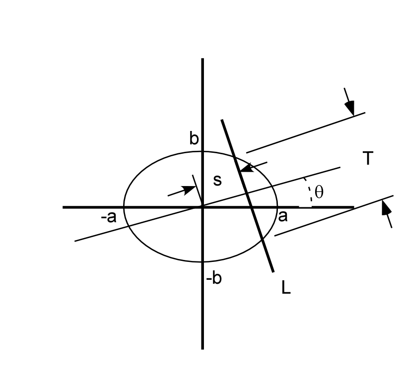
The Matlab radon and iradon tool chain is actually quite unusual. It is more common to specify the object as a set of simple geometric shapes such as ellipsoids each with their own attenuation. The projections are then computed using analytical expressions for the length of intersection of a line with each shape times the attenuation. This is illustrated in Fig. 3↓ for an ellipse. If s is the distance of the line L from the center of the ellipse and θ is the angle from the perpendicular of the line to the principal axis of the ellipse, then the length of the intersection is (see Example 10.2 of Jain [1]).

T = ⎧⎨⎩ 2ab√(s²_m − s²) ⁄ s²_m |s| ≤ s_m 0 |s| > s_m

where s²_m = a²cos²(θ) + b²sin²(θ). The line integral for each line is the sum of the intersection length times the attenuation coefficient of each shape.

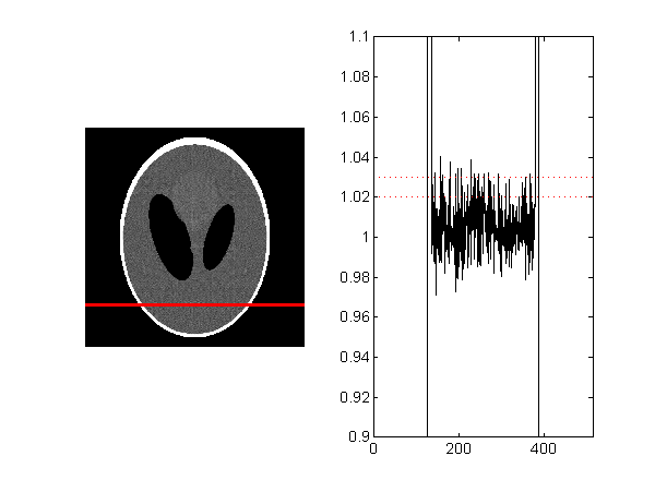
Figure 1 Shepp-Logan phantom with projection data computed with radon and reconstructed with iradon functions. The reconstructed image is on the left. The right panel shows a plot of the image data on the solid red line in the image. Notice the large artifacts do not allow you to see the differences in the reconstructed values.

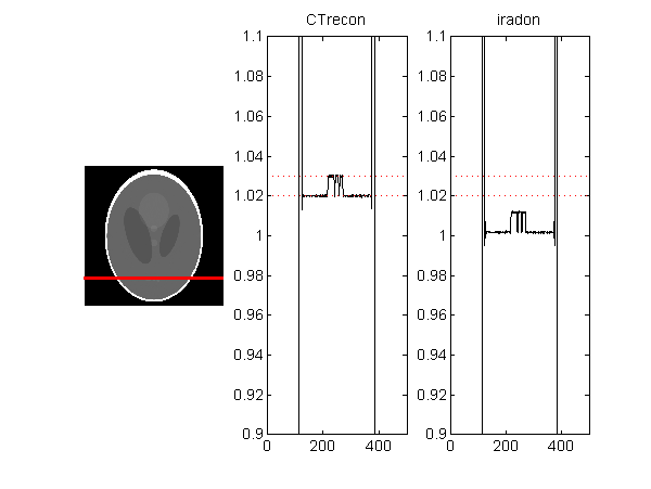
Figure 2 Shepp-Logan phantom with projections computed with my projection simulator and reconstructed with CTrecon. The reconstructed image is on the left; the plot of data along the red line is in the center panel. The right panel shows the same projection data reconstructed with iradon. Note the iradon data are offset from the true levels as noted in my previous post. The red dotted lines in the data plots are at the values of the data inside the “skull” and in the small ellipses.

As shown by the examples, this approach produces data with consistent projections. Another advantage is that it is easily extended to three dimensions. This is more difficult with the image/3D array specification.

A disadvantage of my approach is that it is difficult to use with complex irregular objects. For this, an array based specification may be best but you have to be more sophisticated in the computation than the radon function. In particular, you need to weight the data from each pixel by the length of the line intersection with the pixel. That is not my approach here so I will not discuss it further.

Figure 3 Intersection of line with ellipse.

The simulator program CTsim is written in C++ and the next post discusses some of the utility functions used.

You can download the code used to produce the figures in this post.

Last edited Oct. 4, 2011

Linking is allowed but reposting or mirroring is expressly forbidden.

References

[1] Anil K Jain: Fundamentals of Digital Image Processing. Prentice Hall, 1989.