Click here for a pdf of this post.

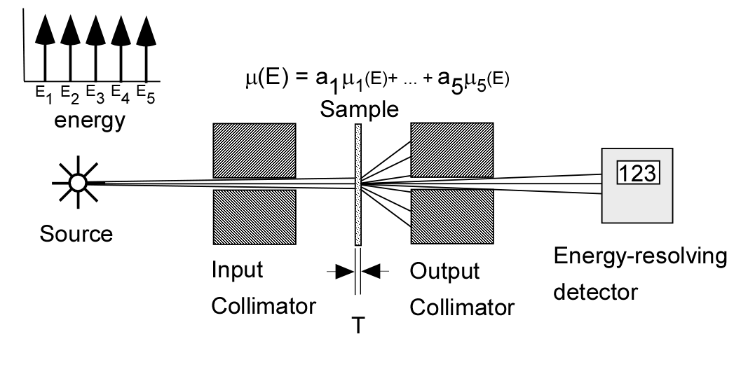
To understand this, consider the experiment shown in Fig. 1↓. We measure the transmitted x-ray photons with a line-spectrum source with an energy-resolving detector. The source has 5 energies E₁, E₂, …, E₅ and the sample consists of varying amounts of 5 different materials with attenuation coefficients μ₁, …, μ₅. The detector counts the number of transmitted photons in 5 energy bins that correspond to the energies of the source. To facilitate the processing, we divide each measurement by the mean number of photons with no object in the beam and then take minus the logarithm

From my discussion in this post (see Eq. 4)

where T is the thickness of the sample. Substituting in (1↑),

Letting A_i = a_iT, we can group L = [L₁, …, L₅]^’ and A = [A₁, …A₅]^’ in vectors to form the matrix equation (the ’ means transpose since I like to work with column vectors)

where μ_i, j = μ_i(E_j).

Eq. 2↑ expresses the fundamental operation of an energy-selective x-ray imaging system. Since the μ_ij are assumed known beforehand, all the information about the object is carried by the A-vector. The fundamental operation of the imaging system is to calculate the A-vector from the measurement L-vector.

With a line-spectrum source, Eq. 2↑ is linear so we can invert the matrix of the μ’s, which I will call M,  multiply times L and then compute A from the measurements

Does this mean that we can make images of as many materials as we want simply by adding more energies? In principle this is possible if the matrix M has full rank. If the entries of M and our measurements L have infinite precision, almost all matrices will have full rank (that is, the rank is equal to the smaller of the number of rows or columns) and we can invert them. However, suppose another matrix with less than full rank is “close” to the original matrix. If the “distance” between the matrices is less than the accuracy of the measurements, then small errors in L will cause much larger errors in A. In this case, the matrix M is effectively not of full rank and Eq. 3↑ is not numerically stable.

We can study this using the concept of numerical or effective rank (Stewart 1973[3]). The theory starts by defining a matrix norm in order to measure “closeness”. The norm is a scalar function of the elements of the matrix which is a measure of its size. For effective rank, the norm is used to measure the difference between the full rank matrix and its lower rank approximating matrix.

The norm can be any function that satisfies the necessary properties of definiteness, homogeneity, and the triangle inequality[3]. A convenient norm can be defined by analogy with a vector norm. The 2-norm for a vector V of length N with components v_i is

The analogous norm for a matrix is called the Frobenius norm. For a matrix B with dimensions M by N, the norm is

A matrix norm defined in this way has all the desirable properties outlined above (Stewart 1973).

The difference between infinite precision and numerical rank can be understood by considering a diagonal matrix, D. The infinite precision rank for this matrix is equal to the number of non-zero entries. The effective rank can also be determined from these values. Suppose we replace the small diagonal entries with zeros. The rank of the modified matrix will be equal to the number of rows or columns minus the number of entries dropped. If the entries are in numerical order and those in columns r + 1 to N are set equal to zero, the difference between the limited accuracy D_a and full precision matrixD, is

If this distance divided by the number of entries is small compared to the error in each of the members, then the effective rank of the original matrix is equal to the rank of the reduced matrix.

Suppose the matrix of interest B is not diagonal. In this case, the singular value decomposition theorem may be applied to transform this case to the diagonal matrix case just described. According to this theorem, there exist unitary matrices U and V such that

where D is a diagonal matrix and V^H is the complex conjugate of the transpose of V.

Since U and V are unitary matrices, multiplying by them does not change the value of the norm. Thus the norms of the original and the diagonal matrices are the same. Suppose the columns of the matrices are rearranged so that the diagonal elements of D are in descending order. Let D_abe the matrix with diagonal entries r + 1 to N equal to zero. The matrix

will have the property that no other matrix of rank r will be closer to B. That is,

is minimum for all matrices of rank r . Thus, depending on the diagonal elements of the matrix D, a matrix of reduced rank may be found which is closer to the original matrix than the error in the terms (with closeness measured in terms of the Frobenius norm). From an experimental point of view, the effective rank of the original matrix is equal to the reduced rank.

The singular values can be calculated by using the singular value decomposition theorem. There are extremely stable numerical methods to compute the SVD so I will use it in the next post to explore the dimensionality of attenuation coefficients.

The SVD is closely related to another tool used to study lower dimension approximations, principal components analysis (PCA). The SVD is more widely known in numerical analysis while PCA is more known in statistics. Statisticians use PCA to “reduce the dimensionality of a data set in which there are a large number of inter-related variables, while retaining as much as possible of the variation present in the data set.”[2]

Suppose the observations are arranged as rows of a matrix X. PCA is implemented by computing the eigenvectors and eigenvalues of the covariance matrix of the data. These have interesting and useful properties (see Ch.1 of Jackson[1]). First, the sum of the eigenvalues is equal to the sum of the variances of the original data. Suppose we arrange the eigenvalues and the corresponding eigenvectors in decreasing order and “center” the data i.e. subtract the averages of the columns from the original data. Then the new variables, the principal components, formed by multiplying the eigenvectors times the columns of the centered data are uncorrelated and each represents the maximum part of the variance of the original data. That is the first principal component represents the maximum part of the variance possible with a single linear transformation of the data. The second represents the maximum part of the remaining variance and so on. Similar to the discussion above, if the distribution of eigenvalues is not uniform, as is often the case, then we can represent most of the variance of the original data by a few principal components.

We can find the relationship between the SVD and PCA as follows. Let X_cbe the centered data. The covariance matrix is C = X^T_cX_c ⁄ n where n is the number of observations i.e. rows in X_c. If W is the matrix of the eigenvectors of C arranged along the columns and Λ is a diagonal matrix of the eigenvalues, then

Using the SVD of the centered data, X_c = UDV^T. I have assumed real data so the Hermitian of a matrix is its transpose, V^H = V^T. Substituting in the definition of the covariance

Since U is unitary, U^TU = I, where I is the identity matrix. Therefore

Comparing Eqs. 10↑ and 12↑, we can see that V is the eigenvectors of the covariance and the square of the singular values divided by the number of observations is equal to the eigenvalues of the covariance.

© 2011 by Aprend Technology and Robert E. Alvarez

Linking is allowed but reposting or mirroring is expressly forbidden.

Edited to add material about principal components.

References

[1] J. Edward Jackson: A User's Guide to Principal Components. John Wiley and Sons, 1991.

[2] Ian T Jolliffe: Principal Component Analysis. Springer-Verlag, 2002.

[3] G. W. Stewart: Introduction to Matrix Computations. Academic Press, 1973.