Cross-section and Attenuation Coefficient

The quantity imaged by x-ray systems is the linear attenuation coefficient, which in turn depends on the cross-sections of x-ray interactions with matter. Here I will discuss the physics of these quantities and will also emphasize the implications for extracting the energy-dependent information.

The interaction of a high energy photon with matter is a lot like a bowling ball going though pins. The initial collision creates a cascade of secondary electrons and photons and sometimes ejects atoms from the lattice. But in the diagnostic x-ray energy region, the interactions are substantially tamer. To the accuracy required for imaging systems design they can be modeled by a cross section: a hypothetical area associated with each atom giving the probability of interaction.

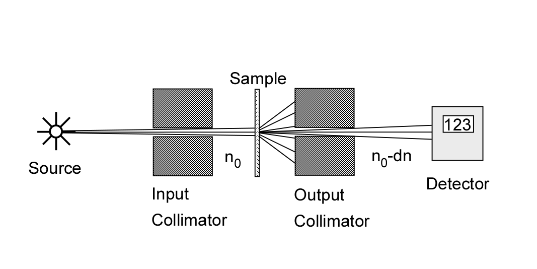
The cross section is defined experimentally as shown in Fig. 1↓. A thin sample of the material is placed between collimators so any interaction removes a photon from the beam. Suppose n photons of energy E are incident on a material of thickness δx with N atoms per unit volume. If, on the average, n − δn photons pass through the material without interacting, then the cross section σ(E) is defined by

(1) (δn)/(n) = − σ(E)Nδx

Note that the cross section has the units of area.

Figure 1 A diagram of an experimental apparatus for measuring the cross section. A collimated beam is incident on the sample and the transmitted photons are collimated so that only those that did not interact are measured by the detector.

Integrating Eq. 1↑, the number that have not interacted after a thickness x will be

(2) n(x) = n₀e^{− σ(E)Nx}

The linear attenuation coefficient is defined to be

(3) μ(E) = σ(E)N

Note that this quantity has the units inverse length m^− 1. If the material composition varies so μ = μ(x, y, z;E), the integral of Eq. (1↑) becomes

(4) n = n₀e^{− ⌠⌡μ(x, y, z;E)ds}

where ∫μ(x, y, z;E)ds is the line integral of the attenuation coefficient of the material on a line from the source to the detector.

Fig. 2↓ shows the attenuation coefficient of some elements as a function of x-ray energy. It is smoothly decreasing except at a small number of step jumps. The energies of the jumps occur near the binding energy of electrons in each shell of the atoms so they are labeled with a spectroscopic notation. The highest energy edge is called the K-edge and it corresponds to the energy required to eject an electron from the innermost shell of the atom. The next highest energy is called the L-edge and so on. Above the K-edge energy, the attenuation coefficient decreases smoothly until it starts to increase above twice the rest mass energy of the electron, 2*512 keV due to pair production. For the relatively low atomic number materials found in the body, the K-edge occurs below the diagnostic energy range.

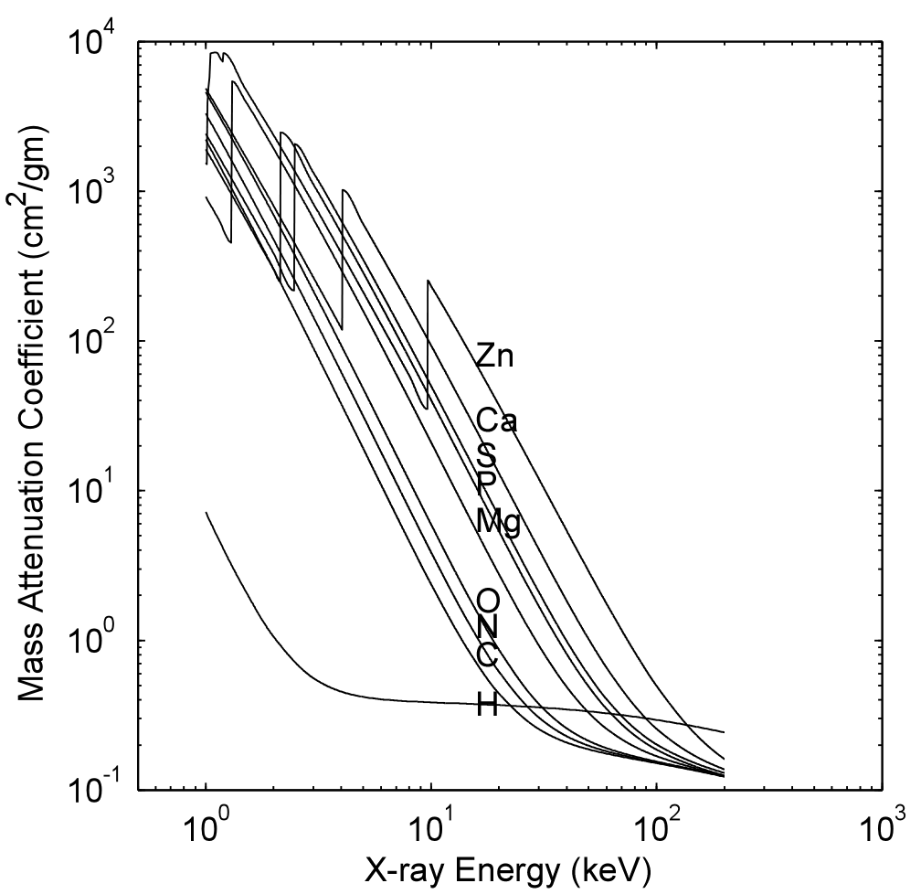
Figure 2 Attenuation coefficients of elements found in the body. The the source code to create this is here

The Mixture Rule

Since the energy of x-rays (more than 10, 000 electron-volts) is much higher than the binding energies of atoms in chemical compounds (1 to 10 electron-volts), the photons interact with the atoms of a material as if they are a mixture of independent atoms irrespective of their chemical state. This rule is useful for computing the attenuation coefficient of compounds and mixtures.

Applying the mixture rule, we can expand the attenuation coefficient at any point r in the object as

μ(r, E) = ^P⎲⎳_i = 1n_i(r)σ_i(E),

where P is the number of chemical elements in the material at each point, n_i(r) the number of atoms, and σ_i(E) the total cross-section of element i. Since the cross-sections are fixed and known before hand, all the information is carried by the coefficients n_i(r). Therefore, we do not need to measure the attenuation at every possible energy. We just need to measure this finite set of at most P constants. Later, we will see that the number of constants required is actually much smaller.

The Sum Rule for X-ray Interactions

X-ray photons interact with matter with only a small number of interaction types. The interactions are classified according to their effects. In Compton scattering, the photon interacts with an electron as if it was not bound to an atom. The direction and energy of the photon change and the electron recoils. In photoelectric absorption, the photon interacts with a tightly bound inner shell electron and the photon disappears and the atom recoils to conserve momentum and is left in an excited state with the energy absorbed from the photon. The final interaction process is coherent or Rayleigh scattering. In Rayleigh scattering, the photon interacts with tightly bound inner shell electrons and the whole atom resonates. The atom then re-emits a photon with the same energy but in a different direction.

The interactions are independent and mutually exclusive so if a photon interacts through one type of process it does not interact through another process. Since the interactions are independent, the probability of not interacting is the product of the probabilities of not undergoing a particular type of interaction

(5) Probability = e^− σ_CNxe^− σ_PNxe^− σ_RNx… = e^{Nx[σ_C + σ_P + σ_R + …]}

where σ_C, σ_P and σ_R are the Compton scattering, photoelectric absorption and Rayleigh scattering cross-sections and x is the thickness of the object. The right side of Eq. (5↑) shows that the total cross section is the sum of the cross sections for the individual interaction types. This is the sum rule.

In general, the three cross-sections depend on the chemical element and the energy. However, if they were separable into multiplicative factors that are functions of atomic number only and of energy only, then the dimensionality is equal to the number of interaction types. That is, if the cross section for an element i with atomic number Z_i is

(6) σ(E, Z_i) = σ_c(E, Z_i) + σ_P(E, Z_i) + σ_R(E, Z_i) + …

and

(7) σ_C(E, Z) = K_C(Z)f_C(E)

(8) σ_P(E, Z) = K_P(Z)f_P(E)

(9) σ_R(E, Z) = K_R(Z)f_R(E)

then

(10) μ(E) = [^N⎲⎳_i = 1n_iK_C(Z_i)]f_C(E) + [^N⎲⎳_i = 1n_iK_P(Z_i)]f_P(E) + [^N⎲⎳_i = 1n_iK_R(Z_i)]f_R(E) + …

Computing the attenuation coefficient

Eq. (10↑) is just suggestive. In order to test it, we need accurate experimental measurements of the attenuation coefficient. Tables for elements and some compounds can be found on the Internet. For example, the US National Institute of Standards and Technology has placed their Report 5632 online (NIST Report 5632). Internet addresses have a very short life span so it best to use a search engine to find the latest address. The data represent the best present estimate and are obtained by judiciously mixing experimental data and theoretical calculations. The NIST 5632 data were incorporated into my function xraymu.m, which will be discussed in the next post.