Estimator for contrast agents-3 Monte Carlo simulation

In this post I continue the discussion of the paper[2], “Efficient, non-iterative estimator for imaging contrast agents with spectral x-ray detectors,” which is available for free download here. The paper extends the previous A-table estimator[1], see this post, to three or more dimension basis sets so it can be used with high atomic number contrast agents. Here I describe the Matlab code to reproduce the figures that summarize the Monte Carlo simulation of the estimators’ performance. The Monte Carlo simulation verifies that the new estimator achieves the Cramèr-Rao lower bound (CRLB) and compares it to an iterative estimator. The simulation code is included with the package for this post.

The Monte Carlo simulation code

The details of the Monte Carlo simulation are described in Sec. II.K of the paper. The simulation computes random samples of a photon counting detector with pulse height analysis and then uses these samples as input to the estimators. It then displays the estimates and their mean squared error (MSE). The MSE is compared with the CRLB.

The simulation code is in the file P62Est3D_3.m included with the code package. It is structured as a set of “code cells,” blocks of code starting with a line with double comment characters %% that can be executed by clicking inside the block in the Matlab editor and then clicking on either the “run section” or “run and advance” icons in the editor commands ribbon. The code has extensive comments so it is (hopefully) fairly easy to understand.

In order to make the simulation more realistic, the calibration data were computed by averaging together 300 random trials. During the trials, the data from a calibrator step in the center of the phantom were also stored and the computational variance of the samples was used in the A-table estimator.

This many exposures is experimentally feasible since each trial corresponds for example to a single exposure at one angle of a CT scan. Since a CT scanner usually acquires over 300 angles during a single scan, which takes only a few seconds in most cases, the calibration data could be acquired rapidly in an experiment.

3D plot of estimates for the three lines

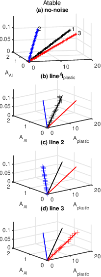
Fig. 1↓ shows three dimensional plots of the estimates from both the A-table and iterative estimators. Each estimator used the same random data as input. The plotted points are the estimates from the first Monte Carlo trial. Notice that the random estimates from both estimators seem quite similar. This is particularly evident with the data for line 3 in the bottom panel (d) of the plots. See Section 4↓ for a quantitative comparison of the estimators’ outputs.

(a)

(b)

Figure 1 3D plot of A-vector estimates for the three lines.

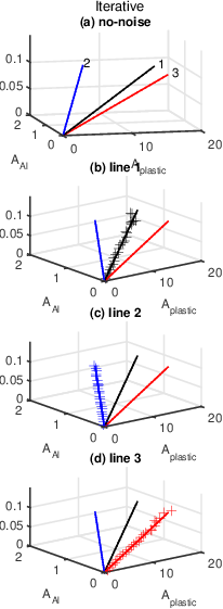
Mean squared errors

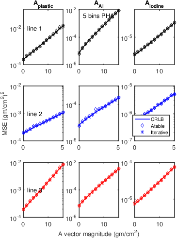
The simulation used the data from 2000 trials to compute the noise variance and mean squared errors. The results with both estimators for each A-vector component on the three lines are shown in Fig. 2↓. Also plotted is the CRLB as the solid lines. The MSE for both estimators are essentially equal to each other and to the CRLB so their symbols overlap except at a few points.

Figure 2 MSE versus CRLB for A-table and Iterative estimators.

Compare A-table and Iterative estimate values

This section compares the two estimators’ outputs quantitatively. The results were not included in the published paper because of space constraints. Fig. 3↓ shows the estimates for line 1 for the first random trial. The left panel shows a 3D plot while the right panel is a plot of the distance between the estimates. The distances are divided by the length of the line to normalize the results and provide a dimensionless quantity. Note that both estimators have essentially the same random variations. The right panel shows that the distance between the two outputs is about 10^− 4 to 10^− 3 of the length of the line in A-space.

(a)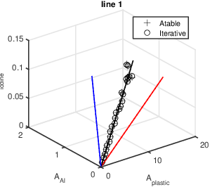

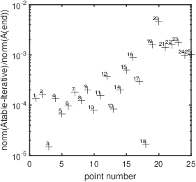
(b)

Figure 3 Plot of A-table and Iterative estimator values on line 1 and normalized distance between them. The estimates are computed with the same random data. The left panel is a 3D plot of the data from both estimators, the + marks the A-table estimates, the o marks the iterative estimator. The right panel shows the distance between the estimators’ output for each point on the line divided by the length of the line. This gives a normalized, dimensionless quantity.

Discussion

Both estimators have mean squared errors close to the CRLB. Since the mean squared error is equal to the sum of the variance and the square of the bias and since the CRLB is the minimum possible variance, MSE values close to the CRLB imply that the bias is negligible and the variance is equal to the CRLB. In estimator theory parlance, the estimators are “efficient.”

Fig. 3↑ shows that the differences of the A-table and iterative estimates are small i.e. they produce essentially the same estimate. The A-table estimator however has the advantages of not requiring x-ray tube spectrum or PHA detector energy response measurements and fast computation in a fixed time.

Last edited Mar 18, 2016

Linking is allowed but reposting or mirroring is expressly forbidden.

References

[1] Robert E. Alvarez: “Estimator for photon counting energy selective x-ray imaging with multi-bin pulse height analysis”, Med. Phys., pp. 2324—2334, 2011. URL http://www.ncbi.nlm.nih.gov/pubmed/21776766.

[2] Robert E Alvarez: “Efficient, non-iterative estimator for imaging contrast agents with spectral x-ray detectors”, IEEE Trans. Med. Imag., 2015. URL http://dx.doi.org/10.1109/TMI.2015.2510869.