If you have trouble viewing this, try the pdf of this post. You can download the code used to produce the figures in this post.
Beam hardening artifacts in CT--the physics of the nonlinearity
Beam hardening artifacts were seen soon after the introduction of CT. Radiologists noticed a ring of increased Hounsfield numbers against the inside of the skull. At first they thought the increase was due to the difference between the white matter in the interior and the gray matter in the cortex of the brain but images of skulls filled with only water also showed the ring so it was obvious the increased values were an artifact.
The EMI corporation, which produced the first CT scanners, must have known about the artifact but they were notoriously close mouthed about the scanner design. In their first scanner the patient stuck his head into a plastic bladder filled with water and the x-ray system measured through the head surrounded by the water. This reduced the dynamic range requirements for the electronics but it also reduced the beam hardening nonlinearity as well as other artifacts as I will show.
In Al Macovski’s group at Stanford, we quickly figured out that the change in average energy of the transmitted photons as the object thickness increases, spectral shift as we called it, would produce a nonlinear relationship between the logarithm of the measurements and the line integral of the attenuation coefficient. We also showed that this nonlinearity could produce the artifact. We were quite interested in it because it was an effect of x-ray energy on the image and we wanted to extract energy dependent information.
Fig. 1↓ shows that the change in average energy and the effective attenuation coefficient as object thickness increases are both quite large. In this post, I will show how this change leads to a nonlinearity between the log of the measurements and the line integral of the object. I will derive expressions for the magnitude of the nonlinearity. These will lead to ways to reduce the nonlinearity and therefore the artifacts. In later posts I will show that the nonlinearity cannot in general be corrected using a lookup table, the no-linearize theorem. I will then describe a general way to understand the effect of the nonlinearity on the reconstructed CT image. Finally, I will examine whether iterative reconstruction methods can be used to correct the artifacts by making the projections and the image consistent.
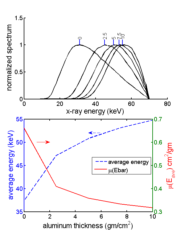
Figure 1 Change in average energy of transmitted photons as object thickness increases. The top panel shows the normalized spectra for different thicknesses of an aluminum object. The spectra were normalized to have the same peak value. The small lines at the tops are at the peak energy values and are labeled by the object thickness. The bottom panel shows the average energy of the spectra (left axis with solid red line) and the aluminum attenuation coefficient at these average energies (right axis, dashed black line) plotted on the same axes.
The beam hardening nonlinearity
A conventional CT scanner, that is, one that does not extract energy information, attempts to reconstruct the object attenuation coefficient at a single average energy, μ(Eave). The quantity that it reconstructs is, to a first approximation,
where Q is the total energy of the transmitted photons and Q0 is the measurement with no object in the beam. With a source photon energy spectrum SQ(E), the transmitted photons’ total energy for a line ℒ through the object Qℒ is
where ∫ℒμ(r, E)dr is the line integral of the attenuation coefficient on the line and r is the geometric position vector. Notice that SQ(E) is not the photon number spectrum used in other posts; it measures the total energy of the photons per unit photon energy.
Suppose the spectrum is a delta function SQ(E) = Q0δ(E − E0). Then Eq. 2↑ becomes
Qℒ = Q0e − ⌠⌡ℒμ(r, E0)dr
and
L = ⌠⌡ℒμ(r, E0)dr.
We can then use a reconstruction algorithm such as convolution-backprojection[1] to reconstruct μ(r, E0).
With a broad spectrum source the delta function model is only an approximation and this will lead to errors. We can model the magnitude of the errors by assuming the object is composed of a single material with a constant density. Then, with the single energy approximation, the line integral of the attenuation coefficient is proportional to the thickness x of the object along the line
(3) L ≈ μ(E0) ⌠⌡ℒdr = μ(E0)x.
If we plot L versus thickness, we should get a straight line through the origin.
Fig. 2↓ shows what happens when we plot L as defined as in Eq. 1↑ with a broad spectrum x-ray tube source spectrum SQ(E) as a function of the object thickness. The value of L is the solid blue line and its curvature is a result of the change in spectrum with thickness shown in Fig. 1↑. The first and second order polynomial approximations to L are also plotted in the figure.
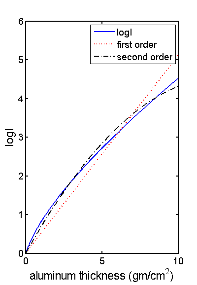
Figure 2 Logarithm of transmitted flux as a function of the object thickness. The actual value of L is the solid blue line. Ideally this would be a straight line but there is nonlinearity due to beam hardening. The dotted red line is a first order least squares approximation and the dashed black line is the second order approximation.
Taylor’s series coefficients
We can use a Taylor’s series to show how the coefficients of the first and second order approximation to Eq. 1↑ depend on the spectrum and the object attenuation coefficient. With a single material, Eq. 1↑ becomes
(4) Q = ⌠⌡SQ(E)e − xμ(E)dE
where x is the thickness of the object and μ(E) is its attenuation coefficient. Expanding L(x) in a Taylor’s series around the origin where L(x) = 0
L(x) = (∂L)/(∂x)(0)x + (∂2L)/(∂x2)(0)x2 + …
Differentiating Eq. 4↑ using this Maxima script,
1/* [ Created with wxMaxima version 12.01.0 ] */ 2 3diff(-log(integrate(S_{Q}(E)*exp(-u(E)*x), E)),x,1); 4 5diff(-log(integrate(S_{Q}(E)*exp(-u(E)*x), E)),x,2);
the first-order coefficient is
(⌠⌡e − x u(E) u(E) S(E)dE)/(⌠⌡e − x u(E) S(E)dE).
This can be re-written as
where Ŝ is the normalized transmitted spectrum
Ŝ = (SQ(E))/(⌠⌡e − xu(E)SQ(E)dE).
The second order coefficient is
(⌠⌡e − x u(E) u(E)2 S(E)dE)/(⌠⌡e − x u(E) S(E)dE) − (⌠⌡e − x u(E) u(E) S(E)dE2)/(⌠⌡e − x u(E) S(E)dE2),
which can be re-written as
Physical interpretation of coefficients
The first order coefficient in Eq. 5↑ is the effective value of the attenuation coefficient using the normalized transmitted spectrum as a weighting function. The second order coefficient in Eq. 6↑ is the “variance” of μ(E) in the normalized spectrum.
Special cases
The nonlinear second order term is zero in at least two cases. The first is when the spectrum is a delta function at E = E0,
(∂2L)/(∂x2)(0)
=
⟨μ2(E)⟩Ŝ − ⟨μ(E)⟩2Ŝ
=
(μ2(E0)) − (μ(E0))2
=
0.
The second case is when the attenuation coefficient μ(E) as a function of energy is a constant, μ0.
(∂2L)/(∂x2)(0)
=
⟨μ2(E)⟩Ŝ − ⟨μ(E)⟩2Ŝ
=
(μ20) − (μ0)2
=
0.
Discussion—the EMI water bladder
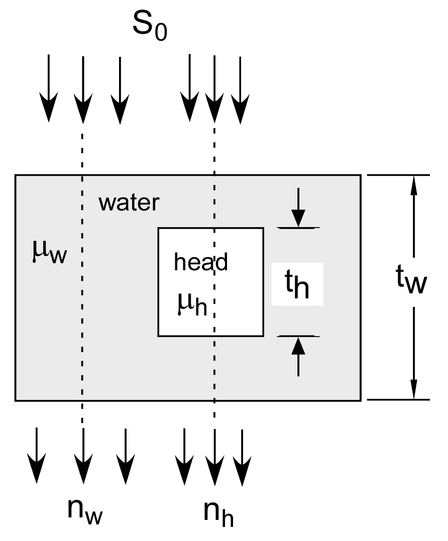
The EMI water bladder, shown in Fig. 3↓, is a clever idea that exploits both of the special cases in the previous Sec. 4↑ to reduce beam hardening artifacts. Suppose the head is composed of a uniform material with attenuation coefficient μh. Then, using the variables defined in the figure, and defining Q0 as the measurement through the water bladder only,
Q0 = ⌠⌡SQ(E)e − twμw(E)dE
the measurement for a line through the head is
Q
=
⌠⌡SQ(E)e − thμh(E) − (tw − th)μw(E)dE
=
⌠⌡[SQ(E)e − twμw(E)]e − th[μh(E) − μw(E)]dE
.
This is equivalent to the measurement through an object with attenuation coefficient equal to the difference between that of the head and water. The measurement is made with a spectrum pre-filtered by the total water bladder thickness.
This does two things to reduce the second order coefficient. The pre-filtering reduces the width of the spectrum thus making it closer to a delta function. The second effect is to reduce the variation of the reconstructed quantity by subtracting the attenuation coefficient of water. Since body materials are mostly made of water, this makes it closer to a constant.
Last edited Jul 04, 2015
Copyright © 2015 by Robert E. Alvarez
Linking is allowed but reposting or mirroring is expressly forbidden.
References
[1] : “Inversion of fan-beam scans in radio astronomy”, The Astrophysical Journal, pp. 427—434, 1967.