A neural net A-vector estimator?

Recently, Zimmerman and Schmidt published a paper[4] comparing the A-table estimator to a neural net estimator. Their main purpose was to compare the estimators with their experimental data but they did mention that they compared the estimators with a simulation. With this, they stated that “Both the neural network and A-table methods demonstrated a similar performance for the simulated data.” This interested me so I decided to compare the estimators using my simulation software to see if I could replicate their results. However, I found that, although the neural network estimator does a great job on no-noise data, with noise it has a substantially larger (about a factor of 100) variance and mean squared error than the A-table estimator. I also compared the estimators with the synthesized attenuation coefficient measure suggested by Zimmerman and Schmidt and found the neural net had about a factor of 10 larger standard deviation, which is consistent with the variance results. I am puzzled about the difference in the results but the code for this post can be used to reproduce the results so any errors or discrepancies can be tracked down.

The background, problem formulation, and notation for A-vector estimators are described in my estimator paper[1] and also here and starting here.

Monte Carlo simulation of A-vector estimator performance

The Monte Carlo simulation is essentially the same as described in my paper[1] except the parameters are adjusted to match those used by Zimmerman and Schmidt. The x-ray tube voltage is 100 kilovolts with 2 × 10⁶ photons incident on the object for each measurement. The object consists of uniform slabs of three materials whose A-vectors lie along the lines shown in Fig. 4↓. As discussed in my dissertation and my “Near optimal ...” paper[2], the A-vectors of different thicknesses of a single material are on a straight line through the origin of A-space where the distance from the origin depends on the thickness and the slope is the ratio of the basis set coefficients.

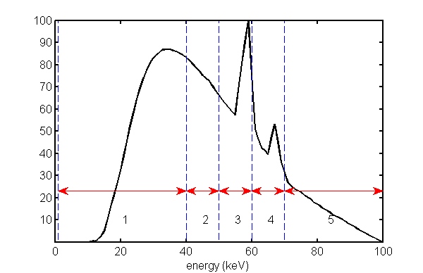
The Monte Carlo simulation generates a set of independent, Poisson distributed random PHA measurements whose expected values are the integrals of the PHA bins and the spectrum transmitted through the object. The interbin energies are the same as those used by Zimmerman and Schmidt. One difference is that their lowest energy bin started at 25 keV while the one used here starts at 0. This was done to avoid re-writing my functions. The difference is small since the lower energies are quickly cut off for any non-zero object thickness. The PHA bins are shown in Fig. 1↓ with the zero thickness spectrum superimposed.

Figure 1 PHA bins with superimposed x-ray tube spectrum. The interbin energies are those used by Zimmerman and Schmidt[4]. The tube spectrum was generated with the TASMIP algorithm[3].

The random PHA data are used to compute estimates of the A-vector for each trial. The same random data are used for each trial with all of the estimators. The statistics for the estimates for each point in the A-space lines are computed and stored in summary arrays and data structures.

The code for the simulation is implemented as a single Matlab script. The script is broken up into Matlab “cells of code” so it can be executed section by section. Of course, the complete script can also be executed to generate all the figures and the data. The random number generator is forced to start in the same state so the same results as shown here can be generated. This is done by the “rng(’default’);” command, which can be removed if different random trials are desired.

The neural network estimator

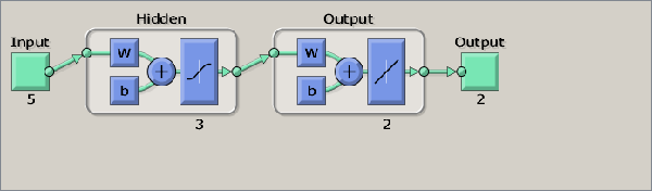
The rationale for the neural network estimator is described in the Zimmerman-Schmidt paper. Their approach was based on one suggested by Lee et al.[5]. It uses the network as function approximator trained with the calibration data. The neural net parameters are random due to the random steps in the optimization so its implementation is “hard-wired” in the code. This is selected by providing the “solvedat” parameter in the call to NeuralNetEstimator function. If this parameter is not present, the neural network will be re-computed using the Matlab Neural Network toolbox functions, as shown in the estimator code. The graphical description of the network is shown in Fig. 2↓.

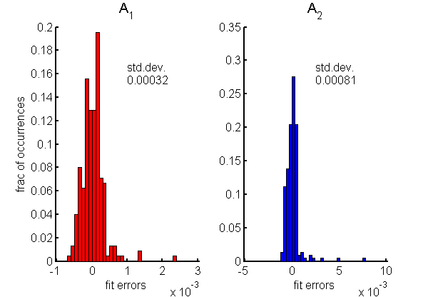
Figure 2 Neural network estimator configuration. This is the graphical description from the Matlab neural network toolbox training function. See the code in my NeuralNetSolve function. Notice that there are 5 inputs, 3 hidden processors, and 2 outputs.

The accuracy of the fit to the calibration data is very good as shown by the histograms of the residuals in Fig. 3↓. Notice that the standard deviation of the errors are of the order of 10^− 4. To put this in context, the A-vector components have a range of 0 to 20 for A₁ and 0 to 1.5 for A₂. These are the errors with no noise data but, as discussed here, the errors with noisy data depend on the estimator used and can be many times larger than these residuals.

Figure 3 Histogram of the neural network approximation errors to the calibration data. Each panel shows the errors in am A-vector component. The standard deviation of the errors is also shown. Notice that they are of the order of 10^− 4 while the components themselves are of the order of 10¹.

The A-table estimator

The A-table estimator is described in detail in my paper[1]. It is implemented in my Matlab function AtableSolveEquations.m.

Plots of estimates vs. actual values

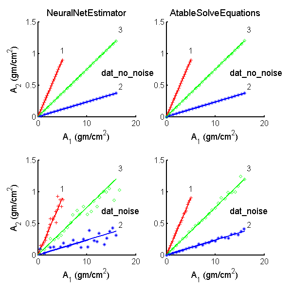
Fig. 4↓ plots the A-vector estimates for the three lines in A-space as discrete points and the actual values as the solid lines. The distances along the lines from the origin correspond to increasing thicknesses of the object. As discussed in Sec. 1↑, both estimators operated on the same data so differences in the values are due to differences in the estimators’ algorithms. The neural net estimator’s outputs are in the left column while the A-table’s are in the right panel. The top row shows the estimates with no-noise data while the bottom row is with noisy data. Notice that both estimators have very low errors with no-noise data but with noisy data the A-table estimator errors are much smaller than the neural net errors.

Figure 4 Comparison of A-vector estimates. The neural net estimator’s estimates are in the left column while the A-table estimates are in the right panel. The top row shows the estimates with no-noise data while the bottom row is with noisy data.

Estimates variance vs. CRLB

Since the spectrum incident on the detectors at each point on the A-space lines (see Fig. 4↑) is known, we can compute the CRLB and plot it along with the mean squared errors (MSE) of the Monte Carlo estimates. Since the MSE is the sum of the variance and the square of the bias and both terms are positive, if it is close to the CRLB, which is the minimum variance, then the estimator is efficient, that is it achieves the CRLB, and has negligible bias. Both estimators had negligible bias compared with the variance so the variance was very close to the MSE.

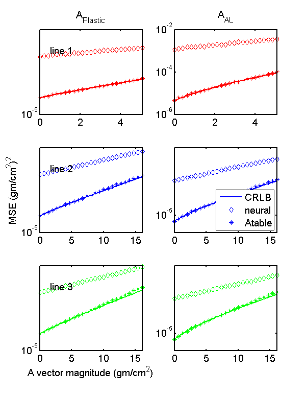
The MSE are computed in the same code section that generates the random data and the results are stored in summary multidimensional arrays. Fig. 5↓ shows the MSE of each of the A-vector components as a function of distance along the lines for the two estimators. The Monte Carlo values are the discrete points while the CRLB is the solid lines. Notice that the A-table MSE is essentially equal to the CRLB except for random fluctuations. Also notice that the neural net MSE is approximately 100 times larger than the A-table results.

Figure 5 Monte Carlo variance as a function of distance along the A-space lines. The Monte Carlo variances with the A-table estimator are the asterisks while the neural net variances are the diamonds. The CRLB variances are the solid lines.

Synthesized attenuation coefficient standard deviation

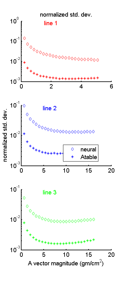
Fig. 6↓ shows the Zimmerman-Schmidt normalized standard deviation or at least my implementation of it. Notice that the neural net value is approximately 10 times larger than the A-table value. This is consistent with the differences in variance in Fig. 5↑.

Figure 6 Synthesized attenuation coefficient standard deviation.

Discussion

These results show that the A-table estimator has lower noise than the neural network estimator. This is contrary to Zimmerman and Schmidt’s conclusion, which is that they are about the same.

A possible explanation is that the neural net implemented here is different than that used by Zimmerman and Schmidt. I made it as close as I could to the implementation described in the paper but there may be some difference. However, the calibration approximation errors in Fig. 3↑ and the estimates in the top row of Fig. 4↑ show that the neural net I used performs well with the no-noise data. The A-table estimator does also. The difference between the estimators is with noisy data.

As I described in my estimator paper[1] and in this post, if there are more measurements than the dimensionality, good estimates with low or no-noise data are not sufficient to guarantee good performance with noisy data. The estimator needs to use information about the probability distribution to handle data that are inconsistent with the many measurements to fewer outputs transformation. The polynomial approximation discussed in the estimator paper and the neural net do not incorporate this information so we would not expect them to do the “right thing” with the inconsistent data.

Last edited Apr 23, 2015

Linking is allowed but reposting or mirroring is expressly forbidden.

References

[1] Robert E. Alvarez: “Estimator for photon counting energy selective x-ray imaging with multi-bin pulse height analysis”, Med. Phys., pp. 2324—2334, 2011. URL http://www.ncbi.nlm.nih.gov/pubmed/21776766.

[2] Robert E. Alvarez: “Near optimal energy selective x-ray imaging system performance with simple detectors”, Med. Phys., pp. 822—841, 2010.

[3] J M Boone, J A Seibert: “An accurate method for computer-generating tungsten anode x-ray spectra from 30 to 140 kV”, Med. Phys., pp. 1661—70, 1997.

[4] Kevin C Zimmerman, Taly Gilat Schmidt: “Experimental comparison of empirical material decomposition methods for spectral CT”, Phys. Med. Biol., pp. 3175, 2015. URL http://dx.doi.org/10.1088/0031-9155/60/8/3175.

[5] Woo-Jin Lee, Dae-Seung Kim, Sung-Won Kang, Won-Jin Yi: “Material depth reconstruction method of multi-energy X-ray images using neural network”, Proc. IEEE Engr. Med. Biol. Conf., pp. 1514-1517, 2012. URL http://dx.doi.org/10.1109/EMBC.2012.6346229.