SNR with pileup-2: Overall plan and NQ detector statistics with pileup

In this post, I continue the discussion of my paper “Signal to noise ratio of energy selective x-ray photon counting systems with pileup”[2], which is available for free download here. The computation of the SNR is based on the approach described in my previous paper, “Near optimal energy selective x-ray imaging system performance with simple detectors[1]”, which is available for free download here. The approach is extended to data with pileup.

The “Near optimal ...” paper shows that regardless whether there is pileup or not, if the noise has a multivariate normal distribution and if the feature is sufficiently thin so the covariance in the background and feature regions is approximately the same, the performance is determined by the signal to noise ratio. So the first thing that has to be done is to show that the data with pileup satisfy these conditions. My plan for the discussion of the SNR paper is therefore as follows.

First, I will use the idealized model and the Matlab function to generate random recorded counts described in the previous post to develop code to compute random samples of data from NQ and PHA detectors with pileup. I will use these functions to derive and validate formulas for the expected values and covariance of the data. These are required to compute the SNR.
I will then use these models and software to determine the conditions so that the probability distribution of the data can be approximated as multivariate normal.
Next, I will show how to use the Cramèr-Rao lower bound (CRLB) to compute the A-vector covariance with pileup data. I will use this to show that we can, under some conditions, use the constant covariance approximation to the CRLB with pileup data just as we can with non-pileup data as shown in this post.
Finally, I will apply these results to compute the reduction of SNR as pileup increases.

In this post, I will use the Matlab function discussed in the previous post to compute random samples of recorded photon counts (N) and total energy (Q) data. These are data from an NQ detector with pileup. I will use these data to validate the formula for the covariance derived in Appendix C of the SNR paper. I will present Matlab code to reproduce Fig. 9 of the paper, which shows the covariance and the correlation of the data as a function of the dead time. I will also use the same data to validate the formulas for the expected value and variance of the recorded counts and the total energy as a function of dead time. These formulas are described in Section 2.E of the paper.

NQ covariance with pileup theory

I derive the formula for the covariance of NQ data in Appendix C of the SNR paper. To test the formula, we can use the function, PileupPulses.m, introduced in the last post to compute random samples of the recorded counts and the total energy during the integration times. The function outputs the recorded counts directly as one of the columns of the counts output variables but does not directly output the total energy. However, it does output the energies of the recorded events, egys_rec, so we can simply sum these to get the total energy.

Software to validate the theoretical model

The code package for this post has the software to create the figures. Some possibly confusing issues:

The PileupPulses.m function requires as an input a sample of random interphoton times, dt_pulse. Because these are random, we do not know how many pulses are required so that the cumulative time is greater than the integration time. The code, shown in the box below, computes the expected value and standard deviation of the number input photons during the integration time and then generates a sample of length equal to the expected value plus 50 times the standard deviation. This reduces the probability of not having enough samples. Samples with times greater than the integration time are just not used. The code to do this is in the “Monte Carlo parameters” code cell block.

1  % compute the required number of input pulses so probability of
2  % "running off end" during the integration time is small
3n_pulses_ave = mean_cps*t_integrate;
4 % input pulses are Poisson distributed so variance = mean
5dev_npulses = sqrt(n_pulses_ave); 
6   % number of pulses to generate to make sure have enough pulses
7npulses2gen =  round(n_pulses_ave+50*dev_npulses);

Another issue is the number of Monte Carlo trials. This determines the variations in the parameters such as the expected values and covariance computed from the random data. The number I used, 2000, was determined by trial and error to give a small enough deviation so we are confident in the validation of the theoretical formulas. The variance and covariance are, by far, more noisy than the expected values.

Results of simulations

Fig. 1↓ shows the expected values and the variances of the recorded photon counts and the total energy as a function of the expected number of photons per dead time, which is equal to the incident rate times the dead time. The results are normalized by dividing by the zero dead time values. Notice that the theoretical model fits the Monte Carlo data well. The expected value and variance of the recorded counts (N) become smaller as the dead time increases but, by the idealized model, the statistics of the total recorded energy(Q) are constant because they do not depend on the dead time.

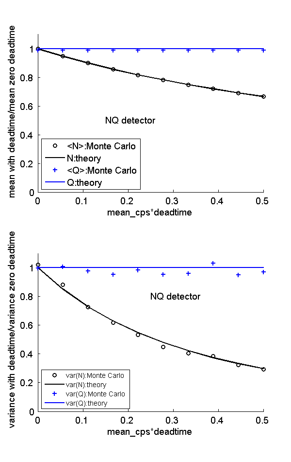
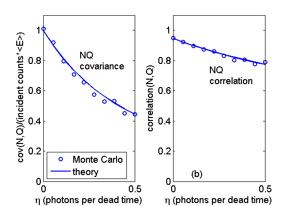
Figure 1 Expected values and the variances of the recorded photon counts and the total energy. The solid lines are the theoretical values and the discrete symbols are the Monte Carlo values. The results are normalized by dividing by the zero dead time values.

Fig. 2↓ shows the covariance and the correlation the N and Q data. The covariance is normalized by dividing by the zero dead time value. Notice that both the covariance and the correlation decrease compared with the zero dead time value. We will see in subsequent posts that this results in a lower SNR.

Figure 2 Covariance and correlation of NQ data. The solid lines are the theoretical values and the discrete symbols are the Monte Carlo values. The covariance is normalized by dividing by the zero dead time value.

Conclusion

The Monte Carlo results are close to the theoretical lines so they validate the formulas.

--Bob Alvarez

Last edited Dec 29, 2014

Linking is allowed but reposting or mirroring is expressly forbidden.

References

[1] Robert E. Alvarez: “Near optimal energy selective x-ray imaging system performance with simple detectors”, Med. Phys., pp. 822—841, 2010.

[2] Robert E. Alvarez: “Signal to noise ratio of energy selective x-ray photon counting systems with pileup”, Med. Phys., pp. -, 2014.