SNR with pileup-1

In the next posts, I will discuss my paper “Signal to noise ratio of energy selective x-ray photon counting systems with pileup”, which is available for free download here. The paper uses an idealized model to derive limits on the effects of pileup on the SNR of A-vector data. There have been many papers (see, for example Overdick et al.[4] Taguchi et al.[3], and Taguchi and Iwanczyk [7]) that use more or less realistic models of photon counting detectors to predict the quality of images computed from their data. These models are necessarily complex since state of the art is relatively primitive compared with the extreme count rate requirements in diagnostic imaging. The complexity of detailed models makes it hard to generalize from the results. Moreover, as research continues, the properties of the detectors will improve and their response will approach an idealized limit. This is the case with the energy integrating detectors used in state of the art medical imaging systems whose noise levels have been reduced so that the principal source of noise is the fundamental quantum noise that is present in all measurements with x-ray photons.

In this post, I will describe the rationale for an idealized model of photon counting detectors with pulse height analysis with pileup and illustrate it with the random data it generates. The following posts will show how the model can be applied to compute the SNR of systems with pileup and to compare the SNR to the full spectrum optimal value. The model will be used to determine the allowable response time so that the reduction in SNR due to pileup is small.

Rationale for the idealized model—errors in photon counting detectors

An example of a fundamental limit in x-ray imaging is quantum noise, which is present in all measurements with electromagnetic radiation. This noise is due to an inherent property of the radiation: in interactions with matter it acts as if it comes in discrete bundles or photons. Photons lead to quantum noise when we measure them over a finite time. Since this noise is due to a property of the radiation, it will be present regardless how small we make the rest of the noise sources in the detector. Therefore, it does not make sense to try to reduce the other noise below the quantum noise limit since this will dominate the performance of the system.

Another fundamental property of the radiation, which is important for photon counters, is that the time between photons is a random quantity. The random properties of photon counts and arrival times can be derived from very general conditions, which simply state that the photon arrivals are statistically independent. There are two ways to define this independence. One was discussed in this post, which gives four conditions to define this independence. Another way is to assert that it is a random counting process where the number of counts N(t) at a time t has the following properties

1) N(0) = 0 2) it has independent increments 3) the number of events in time t is Poisson distributed with mean ρt

where ρ is the rate. Both of these are reasonable and Section 2.2 of Ross[6] shows that the two definitions are equivalent. Either definition leads to results that are consistent with experiments and have been verified in many radiation and nuclear physics experiments.

As discussed by Barrett and Myers[1] in Section 11.1 of their book, the independence conditions require random inter-photon times. As a counter example, suppose the photons arrive at regular times, say once per second. Then the counts would not have independent increments since the probability of increasing the count during the interpulse time is zero and is not independent of a time interval that includes a pulse time, where the probability for increasing the count would always be one. Ross[6] shows that the interpulse times that satisfy the independence conditions are exponential random variables having a mean ¹⁄_ρ.

With the exponential distribution, the probability that the arrival time of the next photon after a given arrival event is greater than t is

P{X₂ > t|X₁ = s} = e^− ρt.

Therefore the probability that one or more photons arrive during the time t is

P{N(t) > 1} = 1 − e^− ρt.

For small times τ, this is approximately ρτ so no matter how small the interval, there is always a non-zero probability of another event. Since any physical detector will have a non-zero response time to process a photon arrival, there will always be the possibility of pulse pileup regardless of how small that time.

Rationale for the idealized model—dead time and recorded counts statistics

It is observed experimentally that as we increase the average rate of photons incident on a counting detector, the recorded counts do not increase linearly. Instead, they tend to saturate and the curve of counts vs. rate drops from the linear increase. In order to explain this behavior in the simplest possible way, two models have been used to describe this behavior using only a single parameter, the dead time. In both models, the detector is assumed to start in a “live” state. With the arrival of a photon the detector enters a separate state where it does not count photons. In the first model, called non-paralyzable , the time in the separate state is assumed to be fixed and independent of the arrival of any other photons during this time. In the second model, called paralyzable, the arrival of photons extends the time in the non-counting state by a fixed time for every arrival. I discussed these in the post mentioned previously.

It is not claimed that the models are realistic descriptions of the operation of real detectors. Instead, like all models, they are simplified versions that try to capture the essential behavior of the detectors in a mathematically tractable form. I chose the nonparalyzable model because it is easier to handle mathematically than the paralyzable model and provides a good fit to the behavior of real detectors. See for example Fig. 5 of Taguchi et al.[3], which shows that the nonparalyzable model fits the experimental data well and fits better than the paralyzable model at high incident photon rates.

Formulas for the mean and variance of the recorded counts as a function of the dead time and the rate of the photons incident on the detector with the nonparalyzable model are derived in the post. They are

⟨N(t)_deadtime⟩ = (ρt)/(1 + ρτ)

Var{N(t)_deadtime} = (ρt)/((1 + ρτ)³)

where ρ is the rate of photons incident on the detector, t is the measurement time, and τ is the dead time. The post also describes and provides the code for a Monte Carlo simulation that validates the formulas.

Rationale for the idealized model—recorded energies

Even without pileup, the recorded energy is not equal to the photon energy due to imperfections in the capture of the photon energy by the detector sensor. The previously cited papers by Overdick et al. and Taguchi and Iwanczyk explain some of the defects that cause errors in the results. A major problem is that the charge pulse created by previous photons has a long duration compared with the interpulse time and prior photon’s pulses may overlap the current photon’s pulse thus distorting the result. Also, other photons may arrive during the current photons’ pulse and their complete pulses may not be measured by the readout electronics. As detector technology improves, the pulses will become shorter and the model I will use goes to the limit and assumes that the recorded energy is the sum of the energies of the photons that occur during the dead time of a pulse regardless of how close the other photons occur to the end of the current photon dead time period.

As noted by Wang et al.[8], this is equivalent to assuming that the pulses for each photon are delta functions with areas equal to their energy. One reviewer of my paper objected that if the pulses are delta functions, there will be no pileup. There are several responses to this seeming conundrum. The first is that even though the pulse shape is narrow, the readout electronics take a finite time to operate introducing a dead time. The second and most important response is that, just as with the paralyzable and nonparalyzable models for counting errors, there is no claim that these models bear any relationship to the actual operation of detectors. Their purpose is to capture the essential behavior of detectors with mathematically tractable equations. The test of the model is how well it fits experiments.

Usefulness of idealized models

The basic assumption that I will make is that these idealized models provide an upper limit to the SNR of real detectors. Obviously, I cannot prove this but it is reasonable to assume that any additional distortions of the data will decrease the SNR. The results will apply to a single measurement so all bets are off if you are, for example, spatially filtering to combine the results from several detectors or making more than one measurement at different times with the same detector and combining the results. Iterative algorithms with “regularity” or smoothness conditions also combine results from different measurements nonlinearly so they will have different SNRs. But in all these cases, having higher quality input data will most likely lead to better final results.

Software for generating random recorded photon counts and energies with pulse pileup

I developed Matlab code to compute recorded photon counts and energies with pulse pileup The non-paralyzable, delta function pulse shape model described in the previous section was used. The computation started by generating random inter-photon times and the energies for photons incident on the detector. The random inter-photon times were generated using the inverse cumulative transform method[5]. For the exponentially distributed inter-photon times of the Poisson process, the inverse cumulative distribution function is the negative of the logarithm so

δt_pulse = − (¹⁄_ρ)log(rand)

where ρ is the expected value of the rate of photons incident on the detector and rand is a uniform (0, 1) random number generator. The photon arrival times are computed as the cumulative sum of the inter-photon times.

The random energies of the photons were derived from the energy spectrum of the photons transmitted through the object without pileup. The spectrum incident on the object was a 120 kilovolt x-ray tube spectrum computed using the TASMIP model[2]. For this post, the object is assumed to have zero thickness.

The recorded counts and energies were computed from the random photon arrival times and energies with the following algorithm. The first photon time started the process. Additional photons with times from the first photon time to that time plus the dead time did not increment the count but did increment the recorded energy. The next photon with time greater than the first photon time plus dead time triggered another recorded count. The recorded energy was computed as with the first photon. The process was repeated for all photon times less than or equal to the integration time of the detector.

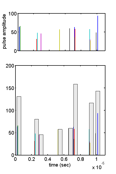
A detailed illustration of the model is shown in Fig. 1↓. The top panel shows photon pulses at random times and with random energies. The bottom panel shows the recorded counts. These are shown by the gray rectangles whose width is equal to the dead time and whose height is equal to the sum of the energies of the pulses during the dead time. The pulses that you generate by running the code will be different from those in the figure since they are random.

Figure 1 Example of pulse pileup model. The top panel shows the pulses occurring at random times and with random energies. The bottom panel shows the recorded pulses and energies. Each recorded pulse is shown by the gray rectangle whose width is the dead time and height is the sum of the pulses occurring during the dead time. If only one pulse occurs the recorded and pulse energy are the same. If more than one pulse occurs, the height is the sum of the energies of the pulses during the dead time. Note the differing y-axis scales of the two subplots.

Conclusion

The rationale for computing the effect of dead time on an energy selective system SNR is discussed. Idealized models are used so that the results represent an upper limit to the performance of physical systems. The code to reproduce the figure is included with the package for this post.

--Bob Alvarez

Last edited Dec 26, 2014

Linking is allowed but reposting or mirroring is expressly forbidden.

References

[1] Harrison H. Barrett, Kyle Myers: Foundations of Image Science. Wiley-Interscience, 2003.

[2] J M Boone, J A Seibert: “An accurate method for computer-generating tungsten anode x-ray spectra from 30 to 140 kV”, Med. Phys., pp. 1661—70, 1997.

[3] Katsuyuki Taguchi, Mengxi Zhang, Eric C. Frey, Xiaolan Wang, Jan S. Iwanczyk, Einar Nygard, Neal E. Hartsough, Benjamin M. W. Tsui, William C. Barber: “Modeling the performance of a photon counting x-ray detector for CT: Energy response and pulse pileup effects”, Med. Phys., pp. 1089—1102, 2011.

[4] Michael Overdick, Christian Baumer, Klaus Jurgen Engel, Johannes Fink, Christoph Herrmann, Hans Kruger, Matthias Simon, Roger Steadman, Gunter Zeitler: “Towards direct conversion detectors for medical imaging with X-rays”, IEEE Trans. Nucl. Sci., pp. 1527—1535, 2008.

[5] Sheldon M. Ross: Simulation, Fourth Edition. Academic Press, 2006.

[6] Sheldon M. Ross: Stochastic Processes. Wiley, 1995.

[7] Katsuyuki Taguchi, Jan S Iwanczyk: “Vision 20/20: Single photon counting x-ray detectors in medical imaging”, Med. Phys., pp. 100901, 2013.

[8] Adam S Wang, Daniel Harrison, Vladimir Lobastov, J Eric Tkaczyk: “Pulse pileup statistics for energy discriminating photon counting x-ray detectors”, Med. Phys., pp. 4265—4275, 2011.