Correlated noise reduction

The noise of the components of the A-vector is highly correlated and the previous post showed a way to produce low noise images analogous to conventional, non-energy selective images by “whitening” the A-vector data. That is good but is there a way to use the correlation to produce lower noise material selective images such as bone or soft tissue canceled? It turns out there are many methods that are seemingly different but are all based on the correlation. Al Macovski introduced the idea and his group at Stanford published several papers on it. It has been used in commercial systems. For example, the Fuji Corporation used an elaborate iterative method to reduce the noise in their “sandwich” photostimulable screen detector system[4]. Other companies like GE are more secretive but I think that they used a similar method with their voltage switching flat panel system. In this post, I will describe a linear least mean squares method, which is a simplified version of the approach introduced by Cao et. al.[2], who also did her work at Stanford. This approach has straight-forward theory, is easy to implement and is effective at reducing noise. One problem with the approach is that it may change the quantitative values of the data in CT and Kalendar et al.[5] published an enhancement that may retain the quantitative information. However, if quantitative data are important, then the software can extract data from the underlying images guided by an operator using the noise-reduced image.

The basic idea

The basic idea is to reduce the noise in a material selective image, S, with a correlated image with lower noise, L. Note that I use the symbol S in a different way than Cao et al. The material selective image might be one of the A-vector components or a bone canceled image computed from low and high voltage images in a dual energy chest x-ray system. The low noise image might be computed as described in the previous post or one of the conventional images in a voltage switched dual energy system. The images are spatially filtered creating low and high frequency pairs for each of the two images.

S = S_l + S_h L = L_l + L_h .

They are then put together to combine the low frequency information from the original material selective image and the estimated high frequency edge information from the low noise image.

Ŝ = S_l + Ŝ_h

Linear least mean square method

The least squares method approaches the problem as one of estimating the high frequency material selective information, S_h, from the correlated high frequency low noise image data, L_h. As the name implies a least squares estimator is used.

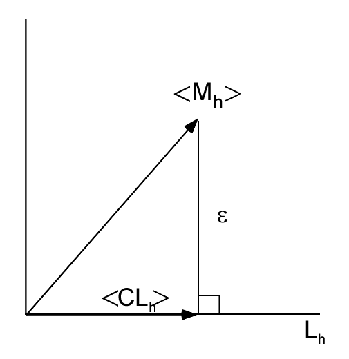
Suppose we model the images as zero mean, two dimensional random processes. Then, at every pixel, we use a linear estimator, Ŝ_h(x, y) = CL_h(x, y), that minimizes the expected value of the error between the estimate and the expected value of the high frequency material selective image data

ϵ = ⟨S_h(x, y) − CL_h(x, y)⟩.

As usual ⟨ ⟩ denotes an expected value.

We can use the orthogonality principle of least squares estimation (see any book on regression analysis such as Ch. 20 of Draper and Smith[3]) to compute the optimal C. We can understand the principle from Fig. 1↓. The minimum error occurs when the ϵ vector is orthogonal to the estimated vector C⟨L_h⟩. When this occurs, the expected inner product is zero:

⟨(S_h(x, y) − CL_h(x, y))L_h(x, y)⟩ = 0.

Multiplying this out

⟨S_hL_h⟩ − C⟨L²_h⟩ = 0.

Solving for C

(1) C = (⟨S_hL_h⟩)/(⟨L²_h⟩).

Figure 1 Orthogonality principle of least squares. The error ϵ = ⟨S_h − CL_h⟩ is minimized when it is orthogonal to L_h.

Estimating C from image data

Of course, we do not know the expected values in the numerator and denominator of Eq. 1↑. But we can estimate them by assuming that the random processes are ergodic over small regions. That is the spatial average is equal to the expected value. Although Cao et al. describe a complex method to estimate C, I have found that a simple method gives good results. The method first computes the image products S_hL_h and L²_h pixel by pixel. Then the products are low pass filtered so that the value at each pixel is the weighted average of the surrounding pixels using the point spread function of the filter as the weights. This gives an approximation to the expected values in Eq. 1↑ so the value of C(x, y) at each pixel can be computed by dividing low pass filtered product images pixel by pixel.

A possible fly in the ointment is that the denominator might be equal to zero. In my code, I tested for that and it did not occur with the images tested. If it did, we could use the values of S_h at those pixels instead of the estimated values.

The Matlab code to implement the algorithm is shown in the code box. Note that the unsharpf function computes the low pass filtered image and subtracts it from the original to give the high pass version so it produces both images at one time. My implementation uses a Gaussian point spread function but others like simple averaging 2D rect functions can also be used.

1[Shigh,sdat] = unsharpf(S,’frac’,frac,’sigma’,sigma);
2Slow = sdat.img_smooth;
3Lhigh = unsharpf(L,’frac’,frac,’sigma’,sigma);
4LSprod = imfilter(Lhigh.*Shigh,sdat.gauss_filt,’replicate’,’conv’);
5LHsq = imfilter(Lhigh.*Lhigh,sdat.gauss_filt,’replicate’,’conv’);
6C = LSprod./LHsq;
7Shat = Slow + C.*Lhigh; % correlated noise filtered image

Example images

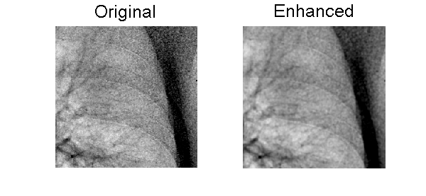
I used the algorithm on some x-ray images made with my “active detector”[1]. This is a dual spectrum detector that combines a storage phosphor sandwich detector with voltage-switched spectra. It results in much better conditioned spectra than a sandwich detector while the voltages can be switch rapidly, within about 100 milliseconds, without moving the storage phosphor screens. The code is included with the package for this post. If you are interested in the raw data for the example, email me.

The filtering parameters were selected ’by hand.’ There may be better ones since I have not done a systematic search. A region of interest extracted from the large original and filtered images is shown in Fig. 2↓.

Figure 2 Example of original (left) and correlation noise filtered image (right).

Conclusion

I have presented the theory and implementation of a correlation noise reduction algorithm for material selective images from x-ray energy spectrum information. Its objective is to reduce noise while retaining edge information.

--Bob Alvarez

Last edited Sep 16, 2014

Linking is allowed but reposting or mirroring is expressly forbidden.

References

[1] R. E Alvarez: “Active energy selective image detector for dual-energy computed radiography”, Med. Phys., pp. 1739—48, 1996.

[2] Qizhi Cao, T. Brosnan, A. Macovski, D. Nishimura: “Least squares approach in measurement-dependent filtering for selective medical images”, IEEE Trans. Med. Imaging, pp. 154—160, 1988.

[3] Norman Richard Draper, Harry Smith: Applied regression analysis. Wiley, 1998.

[4] Wataru Itoh, Kazuo Shimura, Nobuyoshi Nakajima, Masamitsu Ishida, Hisatoyo Kato: “Improvement of detection in computed radiography by new single-exposure dual-energy subtraction”, SPIE Medical Imaging VI, pp. 386—396, 1992.

[5] Willi A Kalender, Ernst Klotz, Lena Kostaridou: “An algorithm for noise suppression in dual energy CT material density images”, IEEE Trans. on Med. Imaging, pp. 218—224, 1988.