The Singular Value Decomposition Approximation Theorem

Not only is the singular value decomposition (SVD) fundamental to matrix theory but it is also widely used in data analysis. I have used it several times in my posts. For example, here and here, I used the singular values to quantify the intrinsic dimensionality of attenuation coefficients. In this post, I applied the SVD to give the optimal basis functions to approximate the attenuation coefficient and compared them to the material attenuation coefficient basis set[1]. All of these posts were based on the SVD approximation theorem, which allows us to find the nearest matrix of a given rank to our original matrix. This is an extremely powerful result because it allows us to reduce the dimensionality of a problem while still retaining most of the information.

In this post, I will discuss the SVD approximation theorem from an intuitive basis. The math here will be even less rigorous than my usual low standard since my purpose is to get an understanding of how the theorem works and what are its limitations. If you want a mathematical proof, you can find it in many places like Theorems 5.8 and 5.9 of the book Numerical Linear Algebra[2] by Trefethen and Bau. These proofs do not provide much insight into the approximation so I will provide two ways of looking at the theorem: a geometric interpretation and an algebraic interpretation.

The SVD approximation theorem

The theorem is:

Let the SVD of a matrix be
(1) B = USV^T
where S is a diagonal matrix with elements greater than or equal to zero and U and V are orthogonal matrices for real data or unitary for complex data. Let S_r be the S matrix with diagonal entries r + 1 to K set equal to zero. The matrix B_r
(2) B_r = US_rV^T

is the closest matrix of rank r to B. That is, the Frobenius norm of the difference of B and B_r is minimum for all matrices of rank r.
(3) ∥B − B_r∥_F = √(^K⎲⎳_{k = r + 1}S²_k) = min_{rank(A) = r}(∥B − A∥_F)

The column space of B is spanned by U so, by the approximation theorem (3↑), the columns of U are the optimal basis vectors. They should be used in the order from largest to smallest singular values since for a given dimension r the first r columns provide the best approximation for that dimension.

geometry: SVD and the action of a matrix

For a geometric interpretation, we can start with a fundamental and useful result proved in Chapter (Lecture) 4 of Trefethen and Bau: if we multiply points on a hypersphere by any matrix the transformed points will lie on a hyperellipsoid. One way to understand this is that, since the elements of a matrix are constants, multiplying by the matrix forms linear combinations of the coordinates of each point. Matrix multiplication is an expansion with constant coefficients so we would expect a smooth distortion of the hypersphere. But why a hyperellipsoid as the result? This is not obvious to me but Trefethen and Bau provide a proof.

We can use use Matlab to verify this result numerically. Fig. 1↓, shows the two dimension case where the hypersphere is a circle. See the caption of the figure for an explanation.

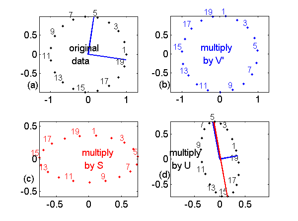
Figure 1 Action of SVD on data on a 2D unit circle centered at the origin. The SVD of the matrix is B = USV^T. The multiplying by B transforms the data to an ellipse. The original data are in Part (a). The effect of multiplying by V^T is in Part (b). The points are labeled in Part (a) so you can see that V^T just rotates the circle but since it is orthogonal it does not distort it. Part (c) shows that multiplying by S scales the axes. Finally, Part (d) shows that multiplying by U rotates the scaled data. The columns of U, plotted as the blue lines, are the semi-axes of the final ellipse. The red line is the full major axis (offset slightly so you can see it). As discussed later, this is the best 1D approximation to the ellipse.

Fig. 2↓ shows the three dimension case. In this case, the 3D hypersphere is a sphere and the points resulting from multiplying by the 3D matrix lie on a 3D ellipsoid.

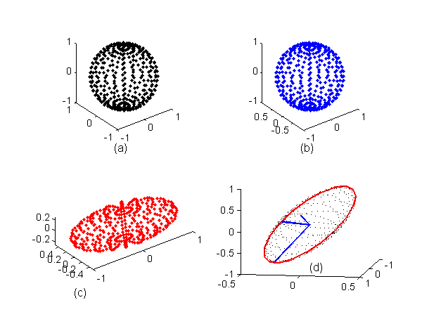
Figure 2 Action of SVD on data on a three dimensional unit sphere, a 3D hypersphere. Again, the result is to transform the hypersphere to a 3D ellipsoid whose semi-axes are the columns of U in the SVD expansion, M = USV^T. The best 2D approximation to the ellipsoid is the ellipse through the largest and 2nd largest axes as shown by the red ellipse in Part (d) of the figure

Geometrical interpretation of the SVD approximation theorem

As I stated in the caption of Fig. 1↑, the columns of U are the axes of the transformed data hyperellipse and the corresponding diagonal elements of S are their lengths. Looking at the transformed data ellipse in Part (d) of Fig. 1↑, we can understand the geometric basis of the SVD approximation theorem in the 2D case. The best one dimensional approximation to the 2D ellipse in Part (d) is the full major axis of the ellipse, from approximately point 5 to 15. This is shown as the red line and is the straight line that minimize the sum or integral of the square of the distances to the ellipse. Similarly, in the 3D case, the best 2D approximation to the 3D ellipsoid in Fig. 2↑ (d) is the ellipse through the centroid with major and minor axes equal to first two columns of U, shown in red in the figure. We can get these semi-axes by setting all elements of S except the first two equal to zero.

We can easily extend this to higher dimensions to find the axes of the closest rank r hyperellipsoids from the columns of U.

Algebraic interpretation: The SVD approximation theorem from diagonal matrices

We can also use algebra to understand the approximation theorem. First, let us see how to find low rank approximations to diagonal matrices. The rank of a diagonal matrix is the number of non-zero elements so to get a lower rank approximation we just set some of the elements equal to zero. As shown in Eq. 4↓, the Frobenius norm of the difference of the original and the reduced rank matrix is the square root of the sum of the squares of the elements that we set equal to zero. We can see that to find the closest lower rank approximation, we sort the diagonal elements so S₁ ≥ S₂ ≥ …S_K and then set to zero the smallest (in absolute value) elements to give us the required reduced rank.

From Parts (b) and (d) of Figs. 1↑ and 2↑, we see that multiplying by an orthogonal (or unitary) matrix is a rigid body rotation that preserves distances between points. Therefore, from the basic SVD Eq. 1↑, the norm of the original matrix is equal to the norm of S. To approximate the original matrix, it makes sense to use the U and V matrices of the original matrix and then to adjust the S matrix. That way we can get the original matrix back for a full rank approximation by using the complete S matrix. By doing this, we can apply the result in Eq. 4↓ to find the optimal lower rank by setting diagonal elements of the full S matrix equal to zero.

(4) ∥∥∥∥∥∥∥⎡⎢⎢⎢⎢⎢⎣ S₁ S₂ S₃ ⋯ ⎤⎥⎥⎥⎥⎥⎦ − ⎡⎢⎢⎢⎢⎢⎣ S₁ 0 0 ⋯ ⎤⎥⎥⎥⎥⎥⎦∥∥∥∥∥∥∥ = √(^K⎲⎳_k = 2S²_k)

Simulation using random matrices

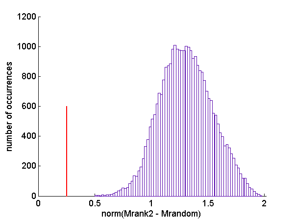
We an test the SVD approximation theorem numerically by generating random lower rank matrices and comparing the norm of the difference with the original matrix to the minimum norm from the SVD. From the code for this article, the original and the lower rank approximations had normally distributed random elements with zero mean and unit variance. Fig. 3↓ shows a histogram of the norm of the differences of the lower rank matrices and the original compared with the difference of the optimal approximation from the SVD. The optimal difference is the red line in the figure. As you can see, even with 30,000 trials, none of the random matrices was closer than the SVD result. There are probably ways to generate random lower rank matrices that are closer to the original but the only ways to do this that occur to me use the SVD approximation theorem.

Figure 3 Histogram of errors with rank 2 matrices compared with minimum error from SVD approximation theorem. The red line is at the minimum error.

Conclusion

The SVD approximation theorem is an important tool that is applicable in many areas so it is important to understand it on an intuitive level. For “big data” computing the SVD can be a problem so an internet search will turn up a lot of work on faster methods to produce low rank approximations but the SVD theorem is the “gold-standard” that these methods are compared to.

--Bob Alvarez

Last edited May 07, 2014

Linking is allowed but reposting or mirroring is expressly forbidden.

References

[1] Robert E Alvarez, Edward J Seppi: “A comparison of noise and dose in conventional and energy selective computed tomography”, IEEE Trans. Nuc. Sci., pp. 2853—2856, 1979.

[2] Lloyd N. Trefethen, David Bau: Numerical Linear Algebra. SIAM, 1997.