Why is polynomial estimator variance so large?

Anyone with experience in energy selective imaging is struck by the terrible performance of polynomial estimators discussed in my last post. This is most likely due to the fact that in the past the number of spectra was almost always equal to the dimension of the A-vector. In this case, as I showed in the last post, any estimator that solves the deterministic, noise free equations is the maximum likelihood estimator (MLE). With equal number of spectra and dimension, the polynomial estimator is accurate for low-noise data so it provides an ’efficient’ estimator. That is its covariance is equal to the Cramèr-Rao lower bound (CRLB). In this post, I examine the reason for the poor performance with more measurements than the A-vector dimension.

Polynomial estimator when number of spectra equal the A-vector dimension

We can see the root cause of the problem from the coverage of the calibration data for noisy data. Fig. 1↓ shows the two measurement spectra—two dimension A-vector case. The black dots are the calibration measurements and the red dots are the measurements with noise for a single A-vector. Notice that the noisy data fall within the calibration region.

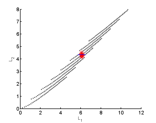
Figure 1 Plot of the calibration data with two spectra. The data are the logI values for a calibration phantom composed of aluminum and plastic with 40 steps from 0 to 5 cm of aluminum and 0 to 30 cm of plastic. The points are subsampled for clarity. The random data for an object with 2 cm of aluminum and 15 cm of plastic are shown as the red dots. Note that the random data are all in the calibration surface. The output of the polynomial and MLE for data on the solid blue line are shown in a later section.

Fig. 2↓ shows the estimates for data on the blue line in Fig. 1↑ The blue curve in Fig. 2↓ is the iterative MLE output and the red curve is the polynomial estimator results. In this case, the outputs are equal verifying the theoretical result from my last post that the polynomial estimator is a maximum likelihood estimator. There are many ways to implement the MLE but, as long as they solve the deterministic equations, they will give the same results.

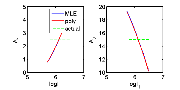
Figure 2 Compare polynomial and MLE estimators for two spectra and two dimension A-vector. Plotted are the output from a MLE (blue line) and the polynomial estimator (red line) for points along the blue line in Fig. 1↑. The two panels are for each component of the A-vector. The outputs of the two estimators are almost equal so the two lines are superimposed.

Polynomial estimator with number of measurement spectra greater than A-vector dimension

The three measurement spectra case is shown in Fig. 3↓. Now the calibration data fall on a two-dimensional surface in the three dimensional measurement space. Deterministically there is no solution for measurements outside the surface. For more measurements than the A-vector dimension, the noisy data, again shown by the red dots in Fig. 3↓, can be off the surface. See the edge-on view in Part (b) of the figure.

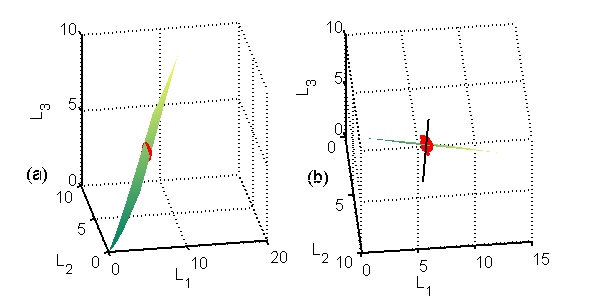
Figure 3 Three dimensional plot of the calibration data with 3 bin PHA. Notice that data only occupy a surface in the 3D space. The left panel (a) shows a view of the surface while in the right panel (b) the view was adjusted so the surface is approximately edge-on. The random data for the 2 cm of aluminum and 15 cm of plastic object are the red dots. Notice that in this case the random data are not all in the calibration surface. The output of the polynomial and MLE are shown in a later section.

Polynomial fit outside the calibration region

Fig. 4↓ shows what happens when we try to use a polynomial fit outside the data region. The figure shows a ninth order fit to the rect function. The fit, plotted as the red line, was calculated with the data from [-1,2]. It gives a fairly good approximation within this region but it diverges rapidly when we try to use it outside this region.

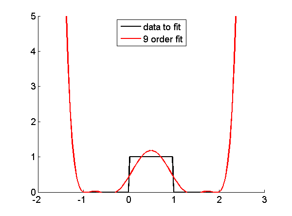
Figure 4 Using polynomial fit outside calibration region. A ninth order polynomial fit was computed to the step function in the region [-1,2]. The red line is the fit function. Notice that the errors are small in the calibration region but rapidly diverge when we use the polynomial approximation outside the region.

Compare MLE and polynomial estimators away from calibration surface

Fig. 5↓ shows the analogous effect for the polynomial estimator. Again the polynomial estimator is the red line and the MLE is the blue line. The polynomial estimator gives the correct value on the calibration surface but rapidly diverges away from it. As a result random measurement data that are not on the surface will produce large values resulting in a much larger variance than the MLE, which gives reasonable results off the calibration surface.

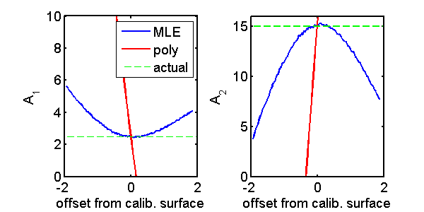
Figure 5 Compare polynomial and MLE estimators for three spectra and two dimension A-vector for points along the perpendicular line to the calibration surface shown in Fig. 3↑. The output from the MLE is the blue line and the polynomial estimator is the red line. The two panels are for each component of the A-vector. The green lines are the actual A-vector values on the surface. Notice that both estimators give the correct results on the calibration surface but the polynomial estimator diverges much more than the MLE for points away from the surface.

Discussion

An important difference between the MLE and the polynomial estimator is that the MLE uses the known probability density function of the measurement data. With this information, the MLE is able to perform reasonably with data that are off the calibration surface and therefore have no deterministic solution. The polynomial estimator does not use this information and based on its mathematical properties it diverges away from the calibration surface. This is responsible for its variance being much larger than the MLE and therefore much larger than the CRLB.

—Bob Alvarez

Last edited Oct 18, 2013

Linking is allowed but reposting or mirroring is expressly forbidden.