If you have trouble viewing this, try the pdf of this post. You can download the code used to produce the figures in this post.
SNR versus tube voltage
In this post, I continue the discussion of my paper, “Near optimal energy selective x-ray imaging system performance with simple detectors.” I summarized many of the theoretical formulas in my last post. Here, I will discuss the formulas for the SNR with x-ray tube spectra with different voltages and different object thicknesses. I will present code to reproduce Figs. 7-9 of the paper. The results show that the energy-selective detectors have SNR that is approximately 4 times larger than the SNR with energy-integrating detectors, the detectors used in almost all conventional medical x-ray systems.
The x-ray detectors
I will compare the performance of 5 different detectors to the ideal detector that measures complete energy spectrum information.
- Q—responds to the total energy of the detected x-ray photons;
- N—counts the total number of detected photons;
- NQ—simultaneously measures the total number and total energy of detected photons;
- N2—two-bin pulse height analysis (PHA);
- N2Q—simultaneous two-bin PHA and integrated energy measurements.
Using the notation in Table 1↓, the ideal SNR with complete energy information is
To evaluate the effective value ⟨f(E)⟩N use the normalized photon number spectrum
(2) n̂(E) = (n(E))/(⌠⌡n(E)dE)
and
Similarly for ⟨f(E)⟩Q,
(4) q̂(E) = (En(E))/(⌠⌡En(E)dE)
and
The code for the ideal SNR in the function OptimalSNR.m (included with the code package) translates Eq. 1↑ directly into Matlab code
d2ideal = mdat.lambda*trapz(sptran.egys,mdat.specnorm.*(sptran.dmus.^2));
% do not divide by 2 or multiply by tf^2 since will do ratio
In this code, trapz is the Matlab trapezoidal numerical integration function, sptran is the data struct for the spectrum transmitted through the object with fields: egys—the photon energies, specnorm—the normalized photon number spectrum, mus is the matrix with background and feature attenuation coefficients, and dmus is the vector of the differences of the mus matrix along the columns.
The matrix formulas for the SNR
where δA = ⟨Afeature⟩ − ⟨Abackground⟩ is the difference between the A vectors in the background and feature region and CA is the covariance of the A vector measurements. The inverse of the A-vector covariance C − 1A is related to the covariance of the logarithm of detector data CL by C − 1A = (MTC − 1LM). Substituting in Eq. 6↑,
(7)
SNR2
=
δATC − 1AδA
=
δATMTC − 1LMδA
By using the attenuation coefficients of the background and feature as the basis functions, δA is the constant vector
δA = ⎡⎢⎣
1
− 1
⎤⎥⎦.
Therefore, to evaluate Eq. 7↑ for the SNR, we need to calculate the detector covariance CL and the effective attenuation coefficient matrix M.
N, Q, and NQ detector
These detectors are simple enough that I was able to evaluate the matrix formulas for the SNR algebraically:
The code from OptimalSNR.m that implements these formulas is:
        % N only
stats.d2N = (mdat.lambda/2)*(trapz(sptran.egys,spnorm(:).*sptran.dmus))^2;
        % Q only
specegy = sptran.egys(:).*spnorm;
specegy_norm = specegy/trapz(sptran.egys,specegy);
stats.d2Q =
(mdat.lambda/(2*mdat.F))*(trapz(sptran.egys,specegy_norm(:).*sptran.dmus))^2;
The SNR using both N and Q signals at the same time, i.e. the NQ detector, is
where F = ⟨E2⟩⁄⟨E⟩2 is the excess variance of the spectrum. This was complex enough that I found it simpler to use the matrix formulation from Eq. 7↑. The code is:
stats.d2NQ = (dA’*mdat.CR_NQinv*dA)/2; % divide by 2 per definition
where mdat.CR_NQinv is computed in CRboundNKQ.m as
CR_NQinv(:,:,kt)= (M_NQ’*inv(RL_NQ)*M_NQ);
and RL_NQ is computed as
          % NQ calcs
    RL_NQ = ones(2); % 2x2
    RL_NQ(2,2) = F;
    RL_NQ = RL_NQ/lambda;
The code for M_NQ evaluates the effective values of the basis set functions, that is the attenuation coefficients of the background and feature materials with the normalized photon number and photon energy using Eqs. 3↑ and 5↑.
Table 1 Symbols
tb
thickness of feature
μb
feature att. coeff.
tf
thickness of background
μf
background att. coeff.
n(E)
photon number spectrum
λ
expected number of photons
E
photon energy
λ
⌠⌡n(E)dE
⟨⟩N
eff. value number spectrum
⟨E⟩k
eff. value of energy spectrum k
μ(E)
a1f1(E) + a2f2(E), linear decomposition
δμ
μf − μb
a1, a2
basis set coefficients
f1(E), f2(E)
basis functions
a
[
a1,
a2
]T
[]T
matrix transpose
A1, A2
basis set coefficient line integrals
A1
⌠⌡ Pa1( r)dr P line, r position
A
[
A1,
A2
]T
A
⌠⌡Pa(r)dr
SNR
signal to noise ratio
CA
covariance of A
I
measurement vector for spectra
L
− log(I⁄I0)
M
matrix of basis funcs. for mnt. spectra
M
(∂L)/(∂A)
SNR of N2 and N2Q detectors vs. inter-bin energy
The SNR of detectors with PHA depends on the inter-bin threshold energy. In my simulations, I optimized the energy to maximize the SNR for each case in the function OptimalSNR.m. The code is shown below:
   % find optimal bin separation idx/energy
idxs4plot = 4:(sptran.negys-4);
  % indexes into sptran.egys array for inter-bin energies
nidxs = numel(idxs4plot);
d2s = zeros(nidxs,2); % columns are SNR2(N2 and N2Q )/SNR2ideal
for kidx = 1:nidxs
    sptran.idx_threshold = idxs4plot(kidx);
    [CR,mdat] = CRboundNKQ(sptran,t_b);
    spnorm = mdat.spec_transmitted/mdat.lambda;
    d2ideal = mdat.lambda*trapz(sptran.egys,mdat.specnorm.*(sptran.dmus.^2));
    % do not divide by 2 or multiply by tf^2 since will do ratio
    d2s(kidx,1) = (dA’*mdat.CR_NKinv*dA)/d2ideal; % N2 — do not divide by 2 since will do ratio
    d2s(kidx,2) = (dA’*mdat.CR_N2Qinv*dA)/d2ideal; % N2Q     "       "
end
The code optimizes by exhaustively computing the SNR with threshold energies throughout the spectrum then selecting the optimum as shown below:
        % N2 is first column of d2s
[d2max,idx] = max(d2s(:,1));
stats.d2N2 = d2max*d2ideal/2;
stats.idx_threshold_N2 = idxs4plot(idx);
stats.Ethreshold_N2 = sptran.egys(stats.idx_threshold_N2);
        % N2Q is 2nd column of d2s
[d2max,idx] = max(d2s(:,2));
stats.d2N2Q = d2max*d2ideal/2;
stats.idx_threshold_N2Q = idxs4plot(idx);
stats.Ethreshold_N2Q = sptran.egys(stats.idx_threshold_N2Q);
The SNR versus inter-bin energy is plotted in Fig. 1↓ for four tube voltages. This should be compared with Fig. 7 of the paper. Although the shapes of the curves are similar the numerical results differ somewhat because the software used to create the figures is not the same. This did not affect the overall conclusions in the following sections.
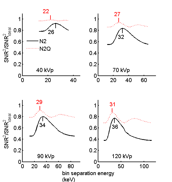
The N2Q SNR changes less with the inter-bin energy than the N2 value. Both of them show more variation as the tube voltage increases.
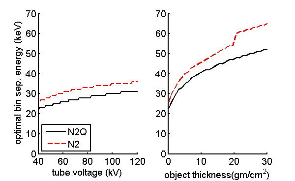
I used the optimal inter-bin energy in the calculations in the following sections since I want to show the best performance of each detector type. In an actual system with PHA detectors, the tube voltage would be fixed but the spectrum will change as the object thickness changes. Fig. 2↓ shows the variation in the inter-bin energy as a function of tube voltage and soft-tissue object thickness. Fig. 5↓ shows the SNR versus thickness with a fixed inter-bin energy. As expected, the SNR drops for thick and thin areas compared with the optimal energy case. This figure is not in the paper but is easy to compute using the code included with this post.
SNR for all detector types
I also used this code to compute the SNR with the five detector types as a function of tube voltage in Fig. 3↓ and versus object thickness in Fig. 4↓. These should be compared with Figs. 9 and 10 of the paper.
Effect of feature material on SNR
added Apr 03, 2013
I will leave it to the reader to modify the code to re-create the figures for an adipose tissue feature. The SNR vs. tube voltage will then be similar to Fig. 11 of the paper. You will see that the results are nearly the same as with a bone material feature. This is due to the fact that the SNR depends on the difference in the attenuation coefficients of the two materials. Compton scattering depends on electron density, which is almost the same for all materials. Therefore the difference with any two materials has a photoelectric interaction energy dependence so the normalized results are nearly the same.
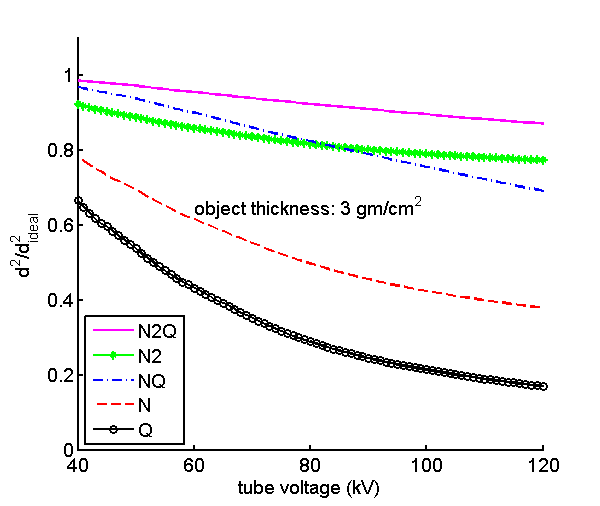
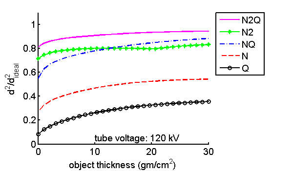
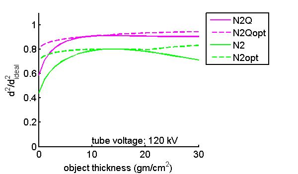
Figure 5 Normalized SNR versus object thickness—fixed vs. optimal inter-bin energy. In Fig. 4↑, the optimal inter-bin energy is used for every object thickness. In this figure, I plot the normalized SNR with a fixed inter-bin energy, 40 and 50 keV for N2Q and N2 detectors respectively. The solid lines are fixed inter-bin energy while the dashed lines are for optimal inter-bin energies that varies for every thickness.
Conclusion
I have described code to reproduce some of the figures in my paper. Although the results differ somewhat in the numerical values the overall conclusions are the same. In general, the SNR divided by the ideal SNR decreases as the spectral width increases because more energy information is available. Nevertheless, the low resolution detectors and especially the N2Q detector can capture a large fraction of the available information. There are some gains with increasing resolution but they are not large.
Last edited Apr 03, 2013
Copyright © 2013 by Robert E. Alvarez
Linking is allowed but reposting or mirroring is expressly forbidden.