If you have trouble viewing this, try the pdf of this post. You can download the code used to produce the figures in this post.
Applying statistical signal processing to x-ray imaging
The last two articles discussed the use of energy information to increase the SNR of x-ray imaging systems. They assumed that the attenuation coefficient is a continuous function of energy and that the energy spectrum is measured with perfect resolution. But we know from my posts here, here, here, and here that the attenuation coefficient can be expressed as a linear combination of two functions of energy. In addition, as I discussed in my posts about deadtime, the extremely high count rates required for medical x-ray systems severely limit the energy resolution and the complexity of the signal processing.
My paper “Near optimal energy selective x-ray imaging system performance with simple detectors[1]”, which is available for free download here, discusses the use of the two-function decomposition in the signal processing. By transforming the problem from infinite to finite dimensions, the decomposition allows us to get near ideal SNR using low energy-resolution measurements, which may be possible with high speed photon counting detectors.
The two-dimensional model allows us to use classical statistical detection and estimation theory (see the books by Van Trees, Detection, Estimation, and Modulation Theory. Part I, and Kay[2]) in the processing. This theory was developed to design communication systems and is based on a three part model. First, an information source produces outputs describable by a small number of constants, such as a 1 or 0 for a binary signal or eight bit bytes. Second, the outputs are transmitted through a communication system and received after being corrupted by random noise described by a probability distribution that depends on the information source outputs. Finally, the receiver computes the best representation of the source outputs from the received data using the random distribution.
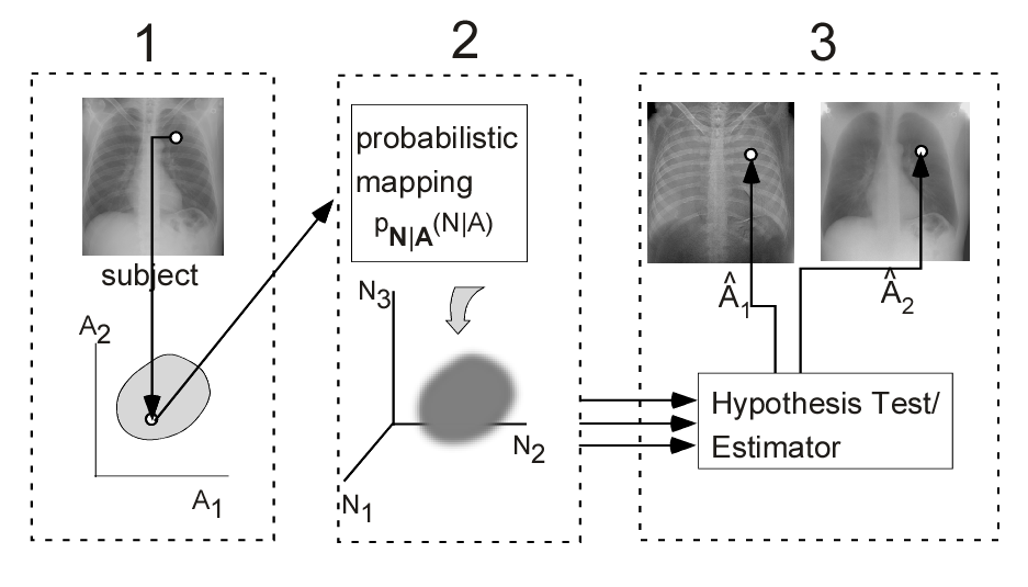
Fig. 1↓ shows the corresponding parts for an x-ray imaging system. In an x-ray system, the information source is the object, whose attenuation is summarized by a finite dimension vector. The object vectors are assumed to be deterministic, i.e. not random, but unknown to us. The object modifies an incident x-ray beam from, for example, an x-ray tube, and the transmitted radiation is measured by a detector producing a vector of data N. The measurements are assumed to be random due to quantum noise and additive electronics noise. They are modeled by a probability distribution pN|A(N|A)) that depends on the source vector A. The statistical processing is carried out by a hypothesis tester or estimator that takes the random data and makes a decision about the object or estimates its A-vector  = [Â1 Â2]T. In the following posts, I will discuss each of the three parts and also show how this model is related to the model used in the last post for the optimal SNR with an energy selective system. In this post, I describe the object model and introduce the noise.
The object
The first part of the signal processing system is a model of the information source--in our case the object. The object x-ray transmission depends on the attenuation coefficient, which is a linear combination of two functions of energy.
(1) μ(E) = a1f1(E) + a2f2(E).
The functions f1(E) and fs(E) are fixed for all materials so they are known beforehand. They therefore do not carry information. The information is summarized by the coefficients a = [
a1
a2
]T. The coefficients summarize everything that we can learn about the object from the transmitted x-rays. With an x-ray system, we cannot measure the coefficients at the three-dimensional points within the object directly. Instead, the transmitted x-rays depend on the line integrals of the coefficients Aj = ∫Saj(r)ds j = 1, 2 along lines from the source to the detector. These coefficients are the components of a vector A. As shown in the first panel of Fig. 1↑, each pixel in the projection image or each line in a CT system data set maps to a point in the two-dimensional A-space.
The random signal model
The transmitted x-rays are measured by a detector producing random signals due to quantum noise, additive electronic noise and other detector imperfections. Quantum noise is the fundamental source and commercial x-ray systems are designed so other noise sources are usually negligible so I will emphasize it in my analysis. With the current state-of-the-art of high speed photon counting detectors, other noise sources and distortions due to pulse pileup can be larger than quantum noise. The goal is quantum limited performance and until this is achieved I do not think they will be widely accepted
X-ray systems measure the object properties by how it affects radiation that is shined on it so the signal has two parts. The first part is a model for the transmitted radiation as a function of the incident radiation and the object properties. The second part is a model for the random errors in the measurements of the transmitted signal. For the first part, I will use a linearized model even though the transmitted signal depends exponentially on the object line integral. I will show that by taking logarithms we can accurately use a linearized model if the noise is small enough.
I will use my usual model: The x-ray source, typically an x-ray tube, produces photons with an energy spectrum ssource(E), which can be either the photon number spectrum n(E) or the photon energy spectrum q(E) = En(E) depending on the type of detector used. The transmitted spectrum at a single energy E is
where ∫μ(r, E)dt is the line integral of the object attenuation coefficient as a function of position within the object r on a line from the x-ray tube focal spot to the detector. Using the basis set decomposition, the line integral can be expressed as
where Ai = ∫ai(r)dt, i = 1, 2. The line integrals A1 and A2 will be considered to be components of a vector A. As I just described, the x-ray imaging system can then be considered to map the object x-ray attenuation onto a set of points in an abstract two-dimensional vector space, which I call the A-plane.
A photon counting detector analyzes the energy of individual photons and counts the number that fall within a set of energy bins during the exposure time. These counts Nk are the integrals of the spectrum of the photons incident on the detector times the effective response function of the bin dk(E). In an idealized model, dk(E) is a rectangle function that is one inside the bin and zero outside but it can also model other responses. Using (2↑), the counts are
Substituting the expression for the line integral (3↑), we can see that the counts are functions of the A vector
(5) Nk(A) = ⌠⌡dk(E)nsource(E)e − A1f1(E) − A2f2(E)dE.
The Nk can be summarized as components of a vector I. There are now two ways to proceed. The first, which is used with counting detectors, assumes that Eq. 5↑ is the mean value of a Poisson random variable and that the data for separate bins are independent. As I discussed in my posts on counting with pulse pileup, this is not true if the deadtime is not negligible. Methods for dealing with this situation are the subject of my current research.
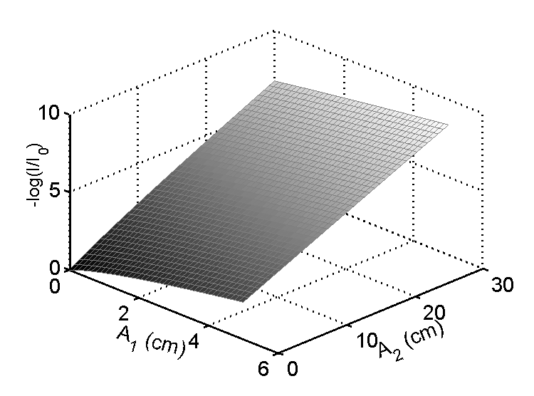
The second way to proceed is to assume that we compute the logarithms of the measurements vector, L = − log(I ⁄ I0), where I0are the data with not object in the beam. The negative is used to give positive quantities since the measurements decrease with increasing object thickness. Fig. 2↓ is a plot of L as a function of A. Notice that the surface is nearly linear with the largest deviation near the origin.
Based on this observation, we can derive a linear model by using a vector Taylor’s series about an operating point A.
Defining δL = L(A + δA) − L(A), the linear model is
(7) δL = (∂L)/(∂A)δA = MδA.
The M matrix is the gradient or slope of the surface in Fig. 2↑. From the figure, it is nearly constant but it does vary somewhat with position in the A-plane. The components of the M matrix can be interpreted as effective attenuation coefficients. Since L = − log(I ⁄ I0), a single component of M = (∂L)/(∂A) , say M11 is
M11 = (∂L1)/(∂A1) = − (1)/(N1)(∂N1)/(∂A1) = (⌠⌡f1(E)dk(E)nsource(E)e − A1f1(E) − A2f2(E)dE)/(⌠⌡dk(E)nsource(E)e − A1f1(E) − A2f2(E)dE).
Notice that (dk(E)nsource(E))/(∫dk(E)nsource(E)e − A1f1(E) − A2f2(E)dE) is the normalized spectrum transmitted through the object, n̂1 so
M11 = ⟨f1(E)⟩n1
The model with noise
Eq. 7↑ is not random. We can introduce noise as an additive term w that depends on the x-ray source energy spectrum, the object, and the detector
δLwith_noise = MδA + w
The noise w is usually modeled as a multivariate normal random vector with the same dimension as L. The mean and the covariance depend on the source spectrum, the object transmission and the type of detector and this will be discussed in my next post.
Last edited Dec 03, 2011
© 2011 by Aprend Technology and Robert E. Alvarez
Linking is allowed but reposting or mirroring is expressly forbidden.
References
[1] : “Near optimal energy selective x-ray imaging system performance with simple detectors”, Med. Phys., pp. 822—841, 2010.
[2] : Fundamentals of Statistical Signal Processing, Volume I: Estimation Theory . Prentice Hall PTR, 1993.