If you have trouble viewing this, try the pdf of this post. You can download the code used to produce the figures in this post.
Monte Carlo simulation of SNR with energy information
In this post, I continue the discussion of my paper “Near optimal energy selective x-ray imaging system performance with simple detectors[1]”, which is available for free download here. I will describe a Monte Carlo simulation of the SNR with energy information discussed in my last post. The simulation traces the paths of individual photons. This is, perhaps, more fundamental than my previous simulations that relied on statistical models for the detector data. I develop models for the random path lengths and use them to simulate the imaging task for SNR described in my last post. The model is validated by comparing the energy spectrum of photons transmitted through an object to the theoretical formula. I also provide an estimate of the errors in the Monte Carlo results.
A good reference for this topic is the book A Monte Carlo Primer by S. A. Dupree and S. K. Fraley[2], although the book is very expensive. I cover all the necessary topics here so the book is not necessary to understand this post but it covers many topics that I do not discuss.
Random path lengths before interaction
As discussed in my previous post, we can describe the probability of a photon interacting with matter by a cross section σ(E), which is defined by
(1) (δn)/(n) = − σ(E)Nδx
In this equation, a thin sample of the material is placed between collimators so any interaction removes it from the beam. If n photons of energy E are incident on a material of thickness δx with N atoms per unit volume., then, on average, n − δn photons pass through the material without interacting. Integrating Eq. 1↑, the number that have not interacted after a thickness x will be
(2) n(x) = n0e − σ(E)Nx
The linear attenuation coefficient is
(3) μ(E) = σ(E)N,
which has the units inverse length m − 1.
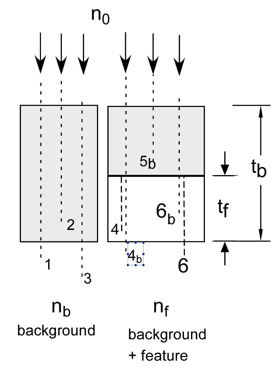
Eq. 2↑ is the same as the probability distribution for the inter-pulse time of a Poisson process discussed here, where the “rate” is μ(E). Notice that the path length distribution depends on the photon energy. Fig. 1↓ shows the geometry and the imaging task. We measure the number of photons nb transmitted through the background region and through a region with background and possibly a feature nf and use the data to decide whether the feature is present.
In the simulation, photons n0 are generated with a specified energy distribution. From the energy E of an individual photon, the attenuation coefficient is calculated and used to generate a random path length
where rand is a uniform (0, 1) random number. The model I use is that any interaction with the material stops the photon so the only ones that get through the background region are those for which t > tb. I also assume that the detector measures all photons that get through the object. These are obviously an oversimplification but they capture the essential features of the problem. In Fig. 1↓, photons 1 and 3 pass through the material but number 2 does not.
The feature region is more complex since it has two materials with different μ(E). There are two ways to approach this problem. One is to express the random path lengths in terms of mean free path (MFP). Then the random paths are simply t = − log(rand) and we can convert the MFP to the actual path length with a function. However the conversion depends on the photon energy so I decided to use an alternate approach. This is a two step process. The first step is the same as for the background-only region. We generate photons, compute their attenuation coefficient and use this to compute a random path length. If this is greater than the thickness of the background material, then we “re-start” the photon at the boundary between the two materials regardless of the actual path length. We compute a new path length using the attenuation coefficient of the feature material and if it is greater than tf the photon is counted. This approach is valid because a Poisson process is “memory less.” The probability of interacting is constant regardless of the position along the path. Once a photon passes the intersection we can compute a new random path starting at the intersection and not affect the results.
Some example photon paths are shown in Fig. 1↓. Photons 4 and 5 are not counted. Although the initial path for photon 4 was greater than tb, the random path length from the intersection is less than tf so the photon does not pass through. The initial path length of photon 5 was less than tb − tf, so it is not counted. Photon 6 is counted because its initial path length is greater than tb − tf and the second path length is greater than than tf .
Simulation implementation
The simulation uses two functions. The first one MakePulses is shown below. First it generates random inter-pulse times, dtpulse and their cumulative times, ttotal. The number of pulses used is the minimum so the cumulative time is greater than the specified integration time t_integrate. The function then generates random energies for these photons using the inverse cumulative transform method discussed in this post.
function [photon_energies,npulse_meas,dtpulse, ttotal] =
MakePulses(mean_cps,t_integrate,spinv,varargin)
% generate enough pulses so total time > t_integrate with high probability
nbar = mean_cps*t_integrate;
npulses2gen = nbar + round(f_excess_pulses*sqrt(nbar)); % generate more for random variations
% make random interpulse times
dtpulse = -(1/mean_cps)*log(rand(npulses2gen,1)); % random interpulse times
ttotal = cumsum(dtpulse);
% use only pulses where ttotal is less than t_integrate
npulse_meas = find(ttotal>t_integrate,1,’first’) - 1;
photon_energies = interp1(spinv.ys, spinv.specuminv, rand(1,npulse_meas) );
Based on the photon energies computed by MakePulses, the function MakePathLengths computes a set of random path lengths. The attenuation coefficient for each energy is computed using linear interpolation by the interp1function. These attenuation coefficients are then used to compute the random path lengths using Eq. 4↑.
function path_lengths = MakePathLengths(photon_energies,mus_struct,nmaterial)
% the mus for each photon energy
mus_photons = interp1(mus_struct.egys, mus_struct.mus(:,nmaterial), photon_energies);
% the path lengths
logrand = -log( rand(1,numel(photon_energies)) );
path_lengths = logrand./mus_photons;
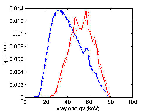
Validate with energy spectra
The software was tested by computing the spectrum of transmitted photons. The relevant code is shown below
%generate the random number of pulses and their energies
photon_energies = MakePulses(mean_cps,30*t_integrate,spinv);
% generate a lot of photons for better stats
path_lengths = MakePathLengths(photon_energies,mus_struct,2);
idx_transmitted = find(path_lengths > tb );
egys_transmitted = photon_energies(idx_transmitted);
The theoretical formula for the spectrum of the transmitted photons is
nb(E) = n0(E)e − μbtb
Fig. 2↓ shows the histograms of the incident and the transmitted photon spectra and the theoretical formulas. The spectra are scaled so they have the same maximum as the histograms. although the transmitted spectra is noisy since there are many fewer photons than the incident spectrum, the Monte Carlo data match the theoretical formulas well.
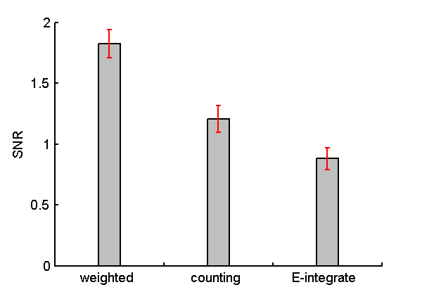
SNR with energy-weighting, photon counting, and energy integrating
A large number of trials were used to compare the SNR with different types of detectors. The SNR was computed as the difference of the mean values in the feature and background region squared divided by the variance of the background region data. The photons transmitted through the feature region were computed using the two step algorithm described above. The relevant code is shown below:
% the feature region — first transmit thru the first part composed of background material
photon_energies = MakePulses(mean_cps,t_integrate,spinv);
% the path lengths — first find those that get through the background material region
path_lengths = MakePathLengths(photon_energies,mus_struct,2); % note 2 for background material
idx_transmitted = find(path_lengths > dthk );
% now find the photons that get through the second part composed of feature material
egys_thru_bk = photon_energies(idx_transmitted);
path_lengths_feature = MakePathLengths(egys_thru_bk,mus_struct,1);% note 1 for feature material
idx_transmitted = find(path_lengths_feature > tf );
The counts weighted with the optimal function described in in my last post were computed as shown below. Since the photons are processed individually, this is just the sum of the weights for the photon energies.
          % each photon occurrence is weighted once
   Nwgtft = sum(interp1(egys,wgts,egys_transmitted));
Fig. 3↓ is a plot of the SNR with each of the detector types. The Monte Carlo results validate the theoretical result
SNR2optimal_wgt ≥ SNR2photon counting ≥ SNR2energy integrating
Discussion
Fig. 3↑ gives an idea of the gain in SNR with complete energy information. The optimal SNR is about twice the energy integrating detector, which is the present state-of-the-art. Since the SNR2 is inversely proportional to the dose, the optimal system can provide the same SNR with less than half the dose. That is a significant advantage and well worth pursuing.
The next step is to develop theory that allows us to compare the SNR with limited energy-resolution detectors to the optimal value and to each other. This will lead me to a discussion of statistical detection theory.
--Bob Alvarez
Last edited Nov 15, 2011
© 2011 by Aprend Technology and Robert E. Alvarez
Linking is allowed but reposting or mirroring is expressly forbidden.
References
[1] : “Near optimal energy selective x-ray imaging system performance with simple detectors”, Med. Phys., pp. 822—841, 2010.
[2] : A Monte Carlo Primer: A Practical Approach to Radiation Transport. Springer, 2001.