If you have trouble viewing this, try the pdf of this post. You can download the code used to produce the figures in this post.
PHA with deadtime—Monte Carlo simulation
I used a Monte Carlo simulation to test the formulas derived in my last post for the mean value, variance, and covariance of pulse height analysis (PHA) data as a function of deadtime. In this post, I discuss the simulation software and the results. The formulas were quite accurate except for the covariance where the relatively small value and the difficulty in getting good statistics for variance estimates in general caused a spread around the theoretical values.
The theoretical formulas
With PHA we measure the energies of the photons and count the number of energies that fall within specified bins. As discussed in my previous post, I model the measured energies as the sum of the initial energy plus the energies of all other photons that occur during the deadtime. The outputs are then the counts Mk in each of the r bins. The bin energies are from [Ek − 1:Ek, k = 1…r]. That is, I idealize the response function to have zero transition width.
From my last post the formulas for the mean value, variance, and covariance of the Mk are
| mean value | ⟨Mk⟩ = ⟨M⟩pk |
| variance | var(Mk) = ⟨M⟩pk + (var(M) − ⟨M⟩)p2k |
| covariance | cov(Mj, Mk) = pjpk(var(M) − ⟨M⟩) |
The variables in these formulas are
| mean total recorded counts | ⟨M⟩ = (λT)/(1 + λτ) |
| variance of recorded counts | var(M) = (λT)/((1 + λτ)3) |
| bin fraction | pk = (∫EkEk − 1Sdeadtime(E)dE)/(∫Sdeadtime(E)dE) |
| spectrum with pulse pileup | Sdeadtime(E) = N0∑∞k = 0((λτ)k)/(k!)e − λτ(s(k)*s) |
| normalized incident spectrum | s(E) = (S(E))/(N0) |
| mean incident counts | N0 = ∫S(E)dE = λT |
| mean incident count rate | λ |
| integration time | T |
| deadtime | τ |
The Monte Carlo simulation is implemented in the function P19Deadtime4.m, included with the code for this post. The main processing is done in the NKQwithDeadtime.c mex function. There is a commented out Matlab implementation of the same code in NKQPileupStats.m that you can use if you do not want to compile the C function. As with my energy spectrum with deadtime post, the calling Matlab function computes the inter-pulse times and the photon energies using the inverse transform method.
The pulse by pulse processing is done in the C code loop shown in the box. There is one iteration of the overall “while” loop for each recorded count. The code first computes the initial pulse time plus the dead time, tend. Then it processes all the subsequent pulses that occur during this time. It adds their energies in the variable egy and finally updates the appropriate bin counter in the array npulses_vec corresponding to the sum of the energies.
// from NKQwithDeadtime.c
// do the processing
tproc = dt_pulse[0]; // the running time as the pulses are processed
while(tproc < t_integrate){
tend = tproc + deadtime; // the end of the deadtime from the current pulse
egy = 0.0; // the energy for this pulse
while( (kpulse<npulses2gen) & (tproc<tend) ){
egy += photon_energies[kpulse];
// Q is the total energy for all pulses including those in deadtimes
Q += photon_energies[kpulse];
kpulse = kpulse + 1;
tproc = tproc + dt_pulse[kpulse];
}
if(kpulse>=npulses2gen){
mexErrMsgTxt("N2QwithDeadtime: overran input dt_pulse array while processing");
}
// update counts for bin corresponding to photon energy
for(kbin =0; kbin<nbins; kbin++){
if( egy < Ethresholds[kbin]){
++npulses_vec[kbin];
break;
}
}
}
Comparison of theoretical and Monte Carlo results
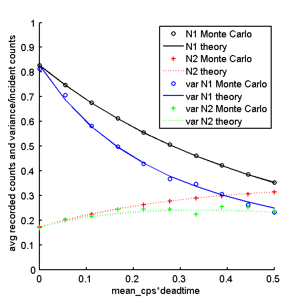
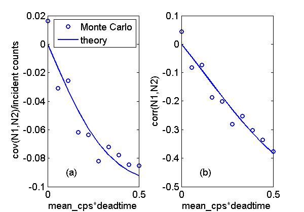
After computing the Monte Carlo data, P19Deadtime4.m computes the Monte Carlo data statistics and the corresponding theoretical values. Fig. 1↓ shows the results for the mean and variance with a two bin PHA system as a function of the deadtime parameter η = λτ. The results are normalized by dividing by the variance of the incident counts. Fig. 2↓ shows the corresponding result for the covariance in Part (a). In Part (b), I plot the correlation, ρ, which is normalized by dividing the covariance by the product of the standard deviations.
ρ = (cov(N1, N2))/(√(var(N1)var(N2)))
Discussion
The theoretical and Monte Carlo results have good agreement for the mean and variance. The covariance values have more variability but are still close to the theoretical results. Notice that, although the covariance in Fig. 2↑(a) seems small, the correlation in Part (b), is close to − 0.4 for larger values of λT. This is a large correlation so the system performance may be substantially affected. In future posts, I will discuss how non-zero deadtime affects energy selective systems using photon counting with PHA.
--Bob Alvarez
Last edited Nov 08, 2011
© 2011 by Aprend Technology and Robert E. Alvarez
Linking is allowed but reposting or mirroring is expressly forbidden.