If you have trouble viewing this, try the pdf of this post. You can download the code used to produce the figures in this post.
Photon Counting with Deadtime-2 The energy spectrum
My previous post discussed the mean and variance of photon counts with deadtime. In this post, I describe a model for the energy spectrum that might be measured by a photon counter with perfect pulse height analysis (PHA). Again, my purpose is to gain insight so I will use a highly simplified model. I derive a theoretical formula for the measured spectrum and then a Monte Carlo simulation to validate the model.
Mathematical model
I will assume that we use a non-paralyzable photon counter. Recall that this means that the arrival of a photon triggers a deadtime period where subsequent photons are not counted. Photons within the deadtime do not extend it so the counter is enabled immediately after the deadtime for the first photon.
Suppose we use PHA to measure the energy of recorded photons. I will assume that the measured energy is the sum of the energies of the incident photons during the deadtime. This model is widely used as a first approximation for example by Taguchi et al.[1] and Wang et al.[3]. These papers extend the model to use more realistic models of the pulse shape but the simplified model retains many of the fundamental effects of deadtime on the measured spectrum.
If the deadtime is very short and and no additional photons arrive, then only the initial photon energy is measured and the spectrum will be that of the incident photons. With a finite deadtime, the energies of the photons that arrive during the deadtime are added to the initial and the measured spectrum shifts towards higher energies. Since the spectrum is averaged over many photon arrivals, we can express it as a sum over conditional probabilities of 0 or more additional photons in the deadtime. In the following sections, I will first derive the energy spectrum of the sum of k photons, then the probability of k photons during the deadtime and finally combine them to derive a formula for the measured energy spectrum.
(1) Sdeadtime(E) = ∞⎲⎳k = 0Sk(E)prob{k}
The energy spectrum of the sum of k photons
Instead of dealing directly with spectra, the derivation is simplified by using the probability density function (PDF) of the photon energies, which is simply the normalized spectrum
p(E) = (S(E))/(N0).
where N0 = ∫S(E)dE. The energies of the individual photons are independent random variables all with a distribution p(E). To derive the PDF of the sum of two energies, we can use the fact that the PDF of the sum of independent random variables is the convolution of their individual PDF’s. A useful way to derive this is to use the characteristic function, which is the Fourier transform of the PDF,
C(w) = ⌠⌡p(v)eiwvdv.
Inspecting the integral, we can see that it is the expected value ⟨eiwv⟩. Now, if the random variables x and y are independent, then ⟨xy⟩ = ⟨x⟩⟨y⟩. This factoring is also valid for functions of the independent random variables, ⟨g(x)h(y)⟩ = ⟨g(x)⟩⟨h(y)⟩. If z = x + y, then its characteristic function is
Cz(w) = ⟨eiw(x + y)⟩ = ⟨eiwxeiwy⟩ = ⟨eiwx⟩⟨eiwy⟩ = Cx(w)Cy(w)
where the last step follows because x and y are independent. Applying the convolution theorem of Fourier transforms
pz = px*py
where the symbol * indicates a convolution.
For k photons, we apply the theorem multiple times to show that
(2) pk(E) = p(k)*p
where p0(E) = p(E). To get the energy spectrum, we multiply by N0 = ∫S(E)dE. Then the spectrum for k photons during the deadtime is Sk(E) = N0p(k)*p.
Probability of k photons during deadtime
I am assuming that the incident counts are a Poisson process. Therefore, the number of counts from the time of the first photon t0 to t0 + τ, where τ is the deadtime is a Poisson random variable with expected value λτ. The probability of k photons during this time is
(3) prob{k} = ((λτ)k)/(k!)e − λτ.
The measured energy spectrum with pulse pileup
Combining Eqs. 2↑ and 3↑ with Eq. 1↑,
This formula is implemented with SpectrumWithPileup.m using the Matlab conv function. The number of terms is chosen so the sum of the terms dropped is negligible.
Monte Carlo simulation software
The simulation works in two steps. First, it generates random interarrival times and energies for the incident photons. Next, it processes the arriving photons one-by-one to compute the recorded photon counts and their energies. The recorded energies are computed using the non-paralyzable model as the sum of all the energies of the initial photon and the photons arriving during the deadtime.
The random variables are computed with the inverse transform algorithm. I will use this often so I discuss it now in some detail. I will use the derivation in sec. 5.1 of Ross, Simulation[2]. The algorithm is based on the following theorem
Let U be a uniform(0, 1) random variable. For any continuous cumulative distribution function (CDF) F, the random variable(5) X = F − 1(U)
has distribution F. The notation F − 1 is the inverse function so F − 1(F(x)) = x.
By definition, the cumulative distribution function of X is
(6)
FX(x)
=
Prob{X ≤ x}
=
Prob{F − 1(U) < x}
where in the last step, I used Eq. 5↑. Since any CDF is monotonically increasing function, we can rewrite any inequality a ≤ b as F(a) ≤ F(b). Therefore the inequality in the last step of Eq. 6↑ is
FX(x)
=
Prob{F(F − 1(U)) ≤ F(x)}
=
Prob{U ≤ F(x)}
=
FU[F(x)]
=
F(x)
where, in the last step, I used the fact that the cumulative distribution function of a uniform random variable is FU(u) = u, 0 ≤ u ≤ 1.
As an example of the use of this theorem, we can generate random photon interarrival times based on the PDF of the exponential random variable
p(δt) = λe − λδt, δt ≥ 0
The cumulative distribution function is F(δt) = λ∫δt0e − λtdt = 1 − e − λδt so its inverse is
F − 1(u) = − (1)/(λ)log(1 − u).
Since 1 − u is also a uniform(0, 1) random variable, we can generate the interarrival times using the Matlab rand function to generate ntimes values
dt_pulse = ( − 1 ⁄ lambda)*log(rand(ntimes, 1)).
With the energy spectrum, we do not have an analytical inverse function but we can use the Matlab cumsum and interp1 functions. See the code for SpectrumCumulativeInverse.m.
The EgysWithPileup.m function uses these formulas to generate random photon interarrival times and the corresponding random photon energies. Then it generates the recorded energies using the following Matlab function. Note the similarity of the function to the CountPulses function of my previous post.
function [egys,Q] = EgysWithDeadtimeLoc(dt_pulse, photon_energies, deadtime, t_integrate)
% output data: egys = the energies of recorded pulses
Q = 0; % total energy of all recorded pulses
egys = -1*ones(numel(dt_pulse),1); %
%pre-allocate for speed. Calling function gets rid of negative values
kpulse = 1; % counter into dt_pulses and photon_energies vectors
tproc = dt_pulse(1); % tproc will increment with each pulse
kegy = 1; % counter into the egys vector
if abs(deadtime) < eps % make sure can increment counter
deadtime = eps; % even with zero deadtime
end
while (tproc < t_integrate) && (kegy<numel(egys))
tend = tproc + deadtime; % initial pulse time + deadtime
egy = 0;
% loop for counts within the deadtime from initial time
while (kpulse<= (numel(dt_pulse)-1) ) && (tproc < tend)
egy = egy + photon_energies(kpulse);
Q = Q + photon_energies(kpulse);
kpulse = kpulse + 1;
tproc = tproc + dt_pulse(kpulse);
end
if kpulse >= (numel(dt_pulse)-1) % make sure do not run off array
return;
end
egys(kegy) = egy;
kegy = kegy+1;
end
Compare Monte Carlo simulation and theoretical formulas
The code for this post has a function to carry out the Monte Carlo simulation. The code computes the random recorded energies with deadtime. Fig. 1↓ shows a comparison of a histogram of the Monte Carlo results and the spectrum computed using Eq. 1↑ for two values of the mean incident counts per second times deadtime η = λτ parameter. The histogram bins are computed in my HistOptBin.m function using the Freedman-Diaconis rule, which is based on number of data points and the inter-quartile range.
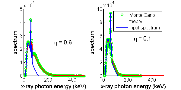
Figure 1 Comparison of theoretical spectrum computed with Eq. 1↑ and histogram of the random energies computed using EgysWithPileup.m for two values of the mean incident counts per second times deadtime η = λτ parameter. The input spectrum is also shown.
Discussion
Deadtime has a strong effect on the measured spectrum smearing it to higher energies than are present in the input spectrum. The data in Fig. 1↑ were computed with parameters η = λτ = 0.6 and 0.1 This is the mean number of incident photons during the deadtime. With high count rates, it is difficult to achieve a low value. For example, if the incident rate is 108 counts per second, then an η ≤ 0.6 implies the deadtime is less than 6 nanoseconds. Taguchi et al.[1] report measured deadtimes of approximately 100 nanoseconds with year 2011 state of the art detectors.
The situation is not as bleak as these numbers indicate because the 108 incident rate is only in the “air” data outside the patient. With the collimation in CT systems, the body transmission in the center can be less than 0.01. In this case, the mean counts per deadtime woud be η = 106*100*10 − 9 = 0.1. As shown in the right panel of Fig. 1↑, the distortion is much smaller in this case. Nevertheless, higher rates are present at the edges of the patient and we need to develop algorithms that can handle the distorted data in these regions.
Last edited Oct. 08, 2011
© 2011 by Aprend Technology and Robert E. Alvarez
Linking is allowed but reposting or mirroring is expressly forbidden.
References
[1] : “Modeling the performance of a photon counting x-ray detector for CT: Energy response and pulse pileup effects”, Med. Phys., pp. 1089—1102, 2011.
[2] : Simulation, Fourth Edition. Academic Press, 2006.
[3] : “Pulse pileup statistics for energy discriminating photon counting x-ray detectors”, Medical Physics, pp. 4265—4275, 2011.