If you have trouble viewing this, try the pdf of this post. You can download the code used to produce the figures in this post. I edited this post on April 27, 2012 to clarify the derivation of the central limit theorem of renewal processes.
Photon Counting with Deadtime-1
The main problem with photon counting detectors in medical x-ray systems is the large count rates, which can be greater than 108 ⁄ sec. The maximum count rate is limited in part by the deadtime and a critical question is the effects of deadtime on the image quality. This post starts the derivation of a simplified model to understand these effects. I do not claim that the model describes a real detector in detail. Instead, I want to get an insight into the magnitude of the effects. For a given mean incident count rate what are small deadtimes that do not affect the results and what values are so large that the images are totally degraded? I start in this post by deriving formulas for the mean value and variance of the recorded counts as a function of deadtime. I found that books and papers that cover this topic, like Parzen[2] and Yu and Fessler[5], refer to other much more mathematical books for the central limit theorem of renewal processes, which forms the basis for the derivation. Here, I present a derivation, which, although decidedly not mathematically rigorous, gives insight into the assumptions of the formulas. I then validate the formulas with a Monte Carlo simulation. As always, I provide the code and data to reproduce the simulation results.
There are many sources of random variations in x-ray measurements but modern detectors are designed so that the random interactions of the radiation with the material of the detector are the limiting factor. Since these are determined by quantum effects, this randomness cannot be removed, so far as we know. These interactions are very complicated involving radiation and material’s properties so we commonly start with an even more simplified mathematical model called the Poisson counting process (see Chs. 2 and 3 of Ross’ book[4]). Some good references for counting detectors are: Ch. 4 of Knoll[3] for the practical details, Ch. 11 of Barrett and Kyle’s book[1] for basic physics as well as photon counting statistics.
Poisson Process
A Poisson counting process with counts N(t) and rate λ describes memoryless random counting. It satisfies the following conditions:
1)
N(0) = 0
2)
it has stationary and independent increments
3)
Prob[N(h) = 1] = λh + o(h)
4)
Prob[N(h) ≥ 2] = o(h)
The first condition just says we start counting at time 0. The second condition is the key property for describing memoryless randomness. With a stationary process, the number of counts depends only on the length of the time interval and not on the absolute time. With independent increments, the counts in non-overlapping time intervals are statistically independent. The third condition defines the count rate: for small intervals the mean number of counts is proportional to the length of the interval. The notation o(h) means a function that decreases faster than linear as h → 0. The fourth condition states that the probability of two or more counts for small intervals is negligible compared to the probability of one count.
All of these are a reasonable assumptions of total randomness. But, of course, no real detector can achieve this ideal. For example, many authors, including Ross[4] and Barrett and Kyle[1], show that these conditions imply that the interarrival time of the events is exponentially distributed. That is, if tn is the arrival time of the n’th event, then the probability that the next event time tn + 1is greater than tn + δt is
(1) Prob(δt) = λe − λδt, δt ≥ 0.
Note this implies that the most probable. i.e. highest probability, δt is zero! The most likely time for the next event to arrive is the previous one. This clearly cannot be true for any physical detector since they always have a finite response time. For later use, we can observe that the mean value of the exponential random variable is 1 ⁄ λ and its variance is 1 ⁄ λ2. Recall that λ is the mean rate so 1 ⁄ λ has the units of time.
Deadtime models
There are several models that are commonly used for the time response of detectors but they are all idealizations. For my purpose, I will choose the non-paralyzable case since this leads to a relatively simple derivation and yet results in the fundamental effects of deadtime. With this model, the effect of the arrival of an event is to put the detector in a non-responsive state for a fixed time. If any other events occur during this deadtime, the count is not incremented. The next event after the end of the deadtime starts the cycle again.
Central limit theorem for renewal processes
In order to derive the statistics with deadtime, we need to do two things: (1) generalize the Poisson process for interarrival time distributions other than exponential, and (2) consider the problem from the point of view of interarrival times in addition to the counts. Step 1 leads to renewal processes. A renewal process is a counting process where the interarrival times are any independent and identically distributed random variables. Step 2 allows us to incorporate deadtime into the model. This is done with the central limit theorem for renewal processes, which allows us to derive the formulas for the mean and variance of counts with deadtime. My derivation here is based on Ross[4].
To see the relationship between counts and interarrival times, we need to focus on the definition of the counting process N(t). This is a set of random variables indexed by the variable t where the experiment for a random variable of this set is the number of events that occur from 0 to t. Suppose, we consider another random variable that is the sum of the first n interarrival times
(2) Tn = n⎲⎳i = 1δtn
where T0 = 0. Then, another way to define N(t) is that it is the largest n such that Tn < t. In mathematical parlance
This can be turned around to see that
In words, (4↑) states that if the number of events counted before time t is less than n then the sum of the first n interarrival times must be greater than t.
We can use this observation to prove the central limit theorem for renewal processes. This theorem states that N(t) is asymptotically (i.e. as t → ∞) normally distributed. In addition, if μ = ⟨δt⟩ is the mean and σ2 = Var(δt) the variance of the interarrival times, δtn, then the asymptotic mean and variance of N(t) are
and
Before I proceed to the proof, let’s examine these formulas. As I mentioned previously, the interarrival times for a Poisson process are exponentially distributed so μ = 1 ⁄ λ and σ2 = 1 ⁄ λ2. Substituting in the mean (5↑) and variance (6↑) formulas, ⟨N(t)Poisson process⟩ → λt and Var{N(t)Poisson process} → λt for large t. This is what we expect for a Poisson random variable.
On to the proof. Using Eq. 2↑, we can see that the expected value of Tn is nμ and, since the δtn are independent, the variance of Tn is nσ2. Applying the central limit theorem to the sum in Eq. 2↑, we can show that as n → ∞
Zn = (Tn − nμ)/(σ√(n)) → N(0, 1)
where N(0, 1) is a normal random variable with mean 0 and variance 1. Therefore
where Φ is the cumulative distribution function of the N(0, 1) random variable
Φ(z) = (1)/(√(2π))z⌠⌡ − ∞e − x2 ⁄ 2dx.
Subtracting and dividing both sides of the inequality N(t) < r , where r = yσ√(t ⁄ μ3) + t ⁄ μ, we can see that
(8) (N(t) − t ⁄ μ)/(σ√(t ⁄ μ3)) < y
is equivalent to N(t) < r, . Applying the alternate definition of N(t) in Eq. 4↑,
Again, subtracting and dividing the inequality Tr > t , we can see that it is equivalent to
Prob{Tr > t} = Prob⎧⎩(Tn − rμ)/(σ√(r)) > (t − rμ)/(σ√(r))⎫⎭ = Prob⎧⎩Zr > (t − rμ)/(σ√(r))⎫⎭.
Substituting the definition of r in the right side, we can see after some algebra that
Since the right hand side approaches − y as t → ∞, the inequality (9↑) for large t is,
Prob⎧⎩(N(t) − t ⁄ μ)/(σ√(t ⁄ μ3)) < y⎫⎭ = Prob{Tr > t} → Prob{Zr > − y} = 1 − Φ( − y)
By the symmetry of the integrand, 1 − Φ( − y) = Φ(y) and this proves the theorem
Prob⎧⎩(N(t) − t ⁄ μ)/(σ√(t ⁄ μ3)) < y⎫⎭ → Φ(y).
Mean and variance of photon counts with deadtime
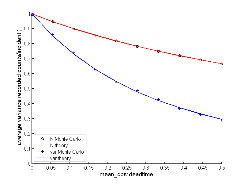
Let us apply the the theorem to the non-paralyzable case with deadtime τ. In this case, the mean interarrival time increases to μdeadtime = 1 ⁄ λ + τ. Since τ is constant, the variance of the interarrival time is unchanged σ2deadtime = 1 ⁄ λ2. The mean and variance of the counts with deadtime are then
As τ → 0, these approach the results for a Poisson process. Note that with finite deadtime, the statistics are no longer Poisson. The variance is somewhat smaller than the mean. This is to be expected since during the deadtimes nothing changes so the variation is somewhat smaller.
Monte Carlo validation of formulas
I wrote a Monte Carlo simulation to test these formulas. For each trial it generates a set of exponentially distributed interarrival times. It then processes the events one by one and counts those that satisfy the non-paralyzable condition. Matlab code to process the events is shown in the box.
function dat_out = CountPulses(dt_pulse,deadtime,t_integrate)
% inputs:
% dt_pulse: the input inter-pulse intervals
% outputs:
% dat = [npulses kpulse];
% npulses: the number of recorded pulses during the integration time
% kpulse: the number of input pulses during the integration time
npulses = 0; % counted pulses
kpulse = 1; % counter into dt_pulses vector
tproc = dt_pulse(kpulse);
while tproc < t_integrate
tend = tproc + deadtime;
while (kpulse<= numel(dt_pulse)) && (tproc < tend)
kpulse = kpulse + 1;
tproc = tproc + dt_pulse(kpulse);
end
npulses = npulses + 1;
end
dat_out = [npulses kpulse];
The results for 10 deadtimes with 10, 000 trials per deadtime are shown in Fig. 1↓. Clearly the theoretical formulas work well.
Discussion
Under what conditions are the asymptotic formulas valid? If we look at the derivation, the key assumption in Eq. 10↑ is that
(yσ)/(√(tμ))≪1.
or
y≪√((μ)/(σ2)t)
Substituting μ = 1 ⁄ λ and σ2 = 1 ⁄ λ2, this is
y≪√(λt)
Now, from Eq. 8↑, y is a “z-score”, i.e. counts normalized by their standard deviation, so it is a number close to one. Therefore, the inequality will be true if the square root of the average number of counts in the measurement time √(λt) is much greater than 1.
Another point is that, for a large signal to noise ratio, smaller variance with large deadtime may seem like a good thing. However, we also have a poorer signal because the missed photons carry information. In upcoming posts, I will study how signal and noise vary with deadtime.
Last edited Oct. 5, 2011. Fixed exponential probability distribution formula. Also, I use the inverse transform method in PileupStats.m to generate exponentially distributed random interpulse times. I will discuss this more in my next post.
© 2011 by Aprend Technology and Robert E. Alvarez
Linking is allowed but reposting or mirroring is expressly forbidden.
References
[1] : Foundations of Image Science. Wiley-Interscience, 2003.
[2] : An Introduction to Probability Theory and Its Applications, Vol. 1. Wiley, 1968.
[3] : Radiation Detection and Measurement. Wiley, 2000.
[4] : Stochastic Processes. Wiley, 1995.
[5] : “Mean and variance of single photon counting with deadtime”, Physics in Medicine and Biology, pp. 2043—2056, 2000.